

|
|
|
|
In Part 13 we saw an example of a Nash equilibrium where both players use a mixed strategy: that is, make their choice randomly, using a certain probability distribution on their set of mixed strategies.
We found this Nash equilibrium using the oldest method known to humanity: we guessed it. Guessing is what mathematicians do when we don't know anything better to do. When you're trying to solve a new kind of problem, it's often best to start with a very easy example, where you can guess the answer. While you're doing this, you should try to notice patterns! These can give you tricks that are useful for harder problems, where pure guessing won't usually work so well.
So now let's try a slightly harder example. In Part 13 we looked at the game 'matching pennies', which was a zero-sum game. Now we'll look at a modified version. It will still be a zero-sum game. We'll find a Nash equilibrium by finding each player's 'maximin strategy'. This technique works for zero-sum two-player normal-form games, but not most other games.
Why the funny word 'maximin'?
In this sort of strategy, you assume that no matter what you do, the other player will do whatever minimizes your expected payoff. This is a sensible assumption in a zero-sum game! They are trying to maximize their expected payoff, but in a zero-sum game whatever they win, you lose... so they'll minimize your expected payoff.
So, in a maximin strategy you try to maximize your expected payoff while assuming that given whatever strategy you use, your opponent will use a strategy that minimizes your expected payoff.
Think about that sentence: it's tricky! But it explains the funny word 'maximin'. In brief, you're trying to maximize the minimum of your expected payoff.
We'll make this more precise in a while... but let's dive in and look at a new game!
In this new game, each player has a penny and must secretly turn the penny to either heads or tails. They then reveal their choices simultaneously. If the pennies do not match—one heads and one tails—B wins 10 cents from A. If the pennies are both heads, player A wins 10 cents from player B. And if the pennies are both tails, player A wins 20 cents from player B
Let's write this game in normal form! If we say
• choice 1 is heads • choice 2 is tails
then the normal form looks like this:
| 1 | 2 | |
| 1 | (10,-10) | (-10,10) |
| 2 | (-10,10) | (20,-20) |
We can also break this into two matrices in the usual way, one showing the payoff for A:
and one showing the payoff for B:
Before we begin our real work, here are some warmup puzzles:
Puzzle 1. Is this a zero-sum game?
Puzzle 2. Is this a symmetric game?
Puzzle 3. Does this game have a Nash equilibrium if we consider only pure strategies?
Puzzle 4. Does this game have a dominant strategy for either player A or player B?
Remember that we write A's mixed strategy as
Here \( p_1\) is the probability that A makes choice 1: that is, chooses heads. \( p_2\) is the probability that A makes choice 2: that is, chooses tails. Similarly, we write B's mixed strategy as
Here \( q_1\) is the probability that B makes choice 1, and \( q_2\) is the probability that B makes choice 2.
Given all this, the expected value of A's payoff is
We saw this back in Part 12.
Now let's actually calculate the expected value of A's payoff. It helps to remember that probabilities add up to 1, so
It's good to have fewer variables to worry about! So, we'll solve for \( p_2\) and \( q_2\):
and write
Then we can calculate A's expected payoff. We start by computing \( A q\):
This gives
This is a bit complicated, so let's graph A's expected payoff in the extreme cases where B either makes choice 1 with probability 100%, or choice 2 with probability 100%.
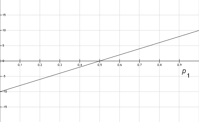
If B makes choice 1 with probability 100%, then \( q_1 = 1.\) Put this in the formula above and we see A's expected payoff is
If we graph this as a function of \( p_1\) we get a straight line:
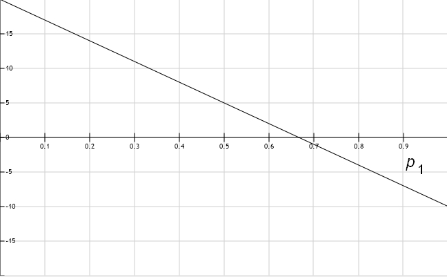
On the other hand, if B makes choice 2 with probability 100%, then \( q_2 = 1\) so \( q_1 = 0.\) Now A's expected payoff is
Graphing this, we get:
The point of these graphs becomes clearer if we draw them both together:
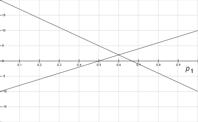
Some interesting things happen where the lines cross! We'll get A's maximin strategy by picking the value of \( p_1\) where these lines cross! And in fact, there's a Nash equilibrium where player A chooses this value of \( p_1,\) and B uses the same trick to choose his value of \( q_1.\)
But we can already see something simpler. We've drawn graphs of A's expected payoff for two extreme cases of player B's mixed strategy: \( q_1 = 1\) and \( q_1 = 0.\) Suppose B uses some other mixed strategy, say \( q_1 = 2/5\) for example. Now A's expected payoff will be something between the two lines we've drawn. Let's see what it is:
If we graph this along with our other two lines, we get this:
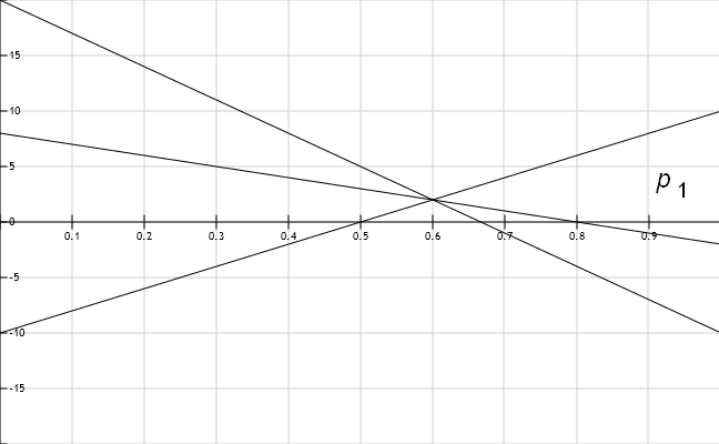
We get a line between the other two, as we expect. But more importantly, all three lines cross at the same point!
That's not a coincidence, that's how it always works. If we draw lines for more different choices of B's mixed strategy, they look like this:

The point where they all intersect looks important! It is. Soon we'll see why.
Now we'll find A's maximin strategy. Let me explain the idea a bit more. The idea is that A is cautious, so he wants to choose \( p_1\) that maximizes his expected payoff in the worst-case scenario. In other words, A wants to maximize his expected payoff assuming that B is trying to minimize A's expected payoff.
Read that last sentence a few times, because it's confusing at first.
Why would B try to minimize A's expected payoff? B isn't nasty: he's just a rational agent trying to maximize his own expected payoff! But if you solved Puzzle 1, you know this game is a zero-sum game. So A's payoff is minus B's payoff. Thus, if B is trying to maximize his own expected payoff, he's also minimizing A's expected payoff.
Given this, let's figure out what A should do. A should look at different mixed strategies B can use, and graph A's payoff as a function of \( p_1.\) We did this:
Then, he should choose \( p_1\) that maximizes his expected payoff in the worst-case scenario. To do this, he should focus attention on the lines that give him the smallest expected payoff:

This is the dark curve. It's not very 'curvy', but mathematicians consider a broken line to be an example of a curve!
To find this dark curve, all that matters are extreme cases of B's strategy: the case \( q_1 = 1\) and the case \( q_1 = 0.\) So we can ignore the intermediate cases, and simplify our picture:
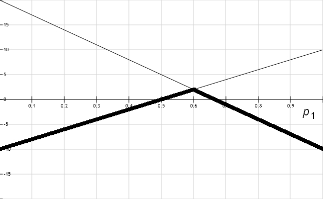
The dark curve is highest where the two lines cross! This happens when
or in other words
So, A's maximin strategy is
It's the mixed strategy that maximizes A's expected payoff given that B is trying to minimize A's expected payoff.
Next let's give the other guy a chance. Let's work out B's expected payoff and maximin strategy. The expected value of B's payoff is
We could calculate this just like we calculated \( p \cdot A q \), but it's quicker to remember that this is a zero-sum game:
so that
and since we already saw that
now we have
To figure out B's maximin strategy, we'll copy what worked for player A. First we'll work out B's expected payoff in two extreme cases:
• The case where A always makes choice 1: \( p_1 = 1.\)
• The case where A always makes choice 2: \( p_1 = 0.\)
We'll get two functions of \( q_1\) whose graphs are lines. Then we'll find where these lines intersect!
Let's get to work. When \( p_1 = 1\) we get
When \( p_1 = 0\) we get
I won't graph these two lines, but they intersect when
or
Hmm, it's sort of a coincidence that we're getting the same number that we got for \( p_1;\) it won't always work this way! But anyway, we see that B's maximin strategy is
Now let's put the pieces together. What happens in a zero-sum game when player A and player B both choose a maximin strategy? It's not too surprising: we get a Nash equilibrium!
Let's see why in this example. (We can do a general proof later.) We have
and
To show that \( p\) and \( q\) form a Nash equilibrium, we need to check that neither player could improve their expected payoff by changing to a different mixed strategy. Remember:
Definition. Given a 2-player normal form game, a pair of mixed strategies \( (p,q),\) one for player A and one for player B, is a Nash equilibrium if:
1) For all mixed strategies \( p'\) for player A, \( p' \cdot A q \le p \cdot A q.\)
2) For all mixed strategies \( q'\) for player B, \( p \cdot B q' \le p \cdot B q.\)
I'll check clause 1) and I'll let you check clause 2), which is similar. For clause 1) we need to check
for all mixed strategies \( p'.\) Just like we did with \( p,\) we can write
We can reuse one of our old calculations to see that
Hmm, A's expected payoff is always 2, no matter what mixed strategy he uses, as long as B uses his maximin strategy \( q!\) So of course we have
which implies that
If you don't believe me, we can calculate \( p \cdot A q\) and see it equals \( p' \cdot A q:\)
Yup, it's 2.
Puzzle 5. Finish showing that \( (p,q)\) is a Nash equilibrium by showing that for all mixed strategies \( q'\) for player B, \( p \cdot B q' \le p \cdot B q.\)
Puzzle 6. How high does this dark curve get?
You have the equations for the two lines, so you can figure this out. Explain the meaning of your answer!
You can also read comments on Azimuth, and make your own comments or ask questions there!
|
|
|
|