Game Theory (Part 20)

John Baez

Last time we tackled von Neumann's minimax theorem:

Theorem. For every zero-sum 2-player normal form game,

\( \displaystyle{\min_{q'} \max_{p'} \; p' \cdot A q' = \max_{p'} \min_{q'} \; p' \cdot A q'}\)

where \( p'\) ranges over player A's mixed strategies and \( q'\) ranges over player B's mixed strategies.

We reduced the proof to two geometrical lemmas. Now let's prove those... and finish up the course!

But first, let me chat a bit about this theorem. Von Neumann first proved it in 1928. He later wrote:

As far as I can see, there could be no theory of games ... without that theorem ... I thought there was nothing worth publishing until the Minimax Theorem was proved.

Von Neumann's gave several proofs of this result:

• Tinne Hoff Kjeldesen, John von Neumann’s conception of the minimax theorem: a journey through different mathematical contexts, Arch. Hist. Exact Sci. 56 (2001) 39–68.

In 1937 he gave a proof which became quite famous, based on an important result in topology: Brouwer's fixed point theorem. This says that if you have a ball

\( B = \{ x \in \mathbb{R}^n : \|x\| \le 1 \}\)

and a continuous function

\( f: B \to B \)

then this function has a fixed point, meaning a point \( x \in B\) with

\( f(x) = x \)

You'll often seen Brouwer's fixed point theorem in a first course on algebraic topology, though John Milnor came up with a proof using just multivariable calculus and a bit more.

After von Neumann proved his minimax theorem using Brouwer's fixed point theorem, the mathematician Shizuo Kakutani proved another fixed-point theorem in 1941, which let him get the minimax theorem in a different way. This is now called Kakutani fixed-point theorem.

In 1949, John Nash generalized von Neumann's result to nonzero-sum games with any number of players: they all have Nash equilibria if we let ourselves use mixed strategies! His proof is just one page long, and it won him the Nobel prize!

Nash's proof used the Kakutani fixed-point theorem. There is also a proof of Nash's theorem using Brouwer's fixed-point theorem; see here for the 2-player case and here for the n-player case.

Apparently when Nash explained his result to von Neumann, the latter said:

That's trivial, you know. That's just a fixed point theorem.

Maybe von Neumann was a bit jealous?

I don't know a proof of Nash's theorem that doesn't use a fixed-point theorem. But von Neumann's original minimax theorem seems to be easier. The proof I showed you last time comes from Andrew Colman's book Game Theory and its Applications in the Social and Biological Sciences. In it, he writes:

In common with many people, I first encountered game theory in non-mathematical books, and I soon became intrigued by the minimax theorem but frustrated by the way the books tiptoed around it without proving it. It seems reasonable to suppose that I am not the only person who has encountered this problem, but I have not found any source to which mathematically unsophisticated readers can turn for a proper understanding of the theorem, so I have attempted in the pages that follow to provide a simple, self-contained proof with each step spelt out as clearly as possible both in symbols and words.

There are other proofs that avoid fixed-point theorems: for example, there's one in Ken Binmore's book Playing for Real. But this one uses transfinite induction, which seems a bit scary and distracting! So far, Colman's proof seems simplest, but I'll keep trying to do better.

The lemmas

Now let's prove the two lemmas from last time. A lemma is an unglamorous result which we use to prove a theorem we're interested in. The mathematician Paul Taylor has written:

Lemmas do the work in mathematics: theorems, like management, just take the credit.

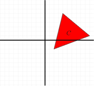
Let's remember what we were doing. We had a zero-sum 2-player normal-form game with an \( m \times n\) payoff matrix \( A\). The entry \( A_{ij}\) of this matrix says A's payoff when player A makes choice \( i\) and player B makes choice \( j\). We defined this set:

\( C = \{ A q' : \; q' \textrm{ is a mixed strategy for B} \} \subseteq \mathbb{R}^m \)

For example, if

\( \displaystyle{ A = \left( \begin{array}{rrr} 2 & 10 & 4 \\-2 & 1 & 6 \end{array} \right) } \)

then \( C\) looks like this:

We assumed that

\( \displaystyle{ \min_{q'} \max_{p'} \; p' \cdot A q' > 0} \)

This means there exists \( p'\) with

\( \displaystyle{ p' \cdot A q' > 0} \)

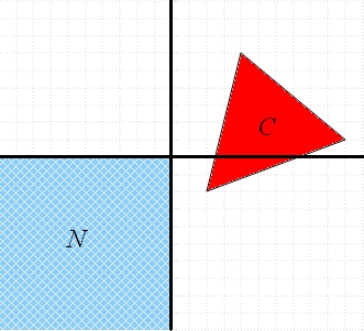
and this implies that at least one of the numbers \( (Aq')_i\) must be positive. So, if we define a set \( N\) by

\( \displaystyle{ N = \{(x_1, \dots, x_m) : x_i \le 0 \textrm{ for all } i\} \subseteq \mathbb{R}^m }\)

then \( Aq'\) can't be in this set:

\( \displaystyle{ Aq' \notin N }\)

In other words, the set \( C \cap N\) is empty.

Here's what \( C\) and \( N\) look like in our example:

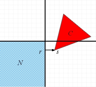
Next, we choose a point in \( N\) and a point in \( C\):

• let \( r\) be a point in \( N\) that's as close as possible to \( C,\)

and

• let \( s\) be a point in \( C\) that's as close as possible to \( r,\)

These points \( r\) and \( s\) need to be different, since \( C \cap N\) is empty. Here's what these points and the vector \( s - r\) look like in our example:

To finish the job, we need to prove two lemmas:

Lemma 1. \( r \cdot (s-r) = 0,\) \( s_i - r_i \ge 0\) for all \( i,\) and \( s_i - r_i > 0\) for at least one \( i.\)

Proof. Suppose \( r'\) is any point in \( N\) whose coordinates are all the same those of \( r,\) except perhaps one, namely the \( i\)th coordinate for one particular choice of \( i.\) By the way we've defined \( s\) and \( r\), this point \( r'\) can't be closer to \( s\) than \( r\) is:

\( \| r' - s \| \ge \| r - s \| \)

This means that

\( \displaystyle{ \sum_{j = 1}^m (r_j' - s_j)^2 \ge \sum_{j = 1}^m (r_j - s_j)^2 } \)

But since \( r_j' = r_j\) except when \( j = i,\) this implies

\( (r_i' - s_i)^2 \ge (r_i - s_i)^2 \)

Now, if \( s_i \le 0\) we can take \( r'_i = s_i.\) In this case we get

\( 0 \ge (r_i - s_i)^2 \)

so \( r_i = s_i.\) On the other hand, if \( s_i > 0\) we can take \( r'_i = 0\) and get

\( s_i^2 \ge (r_i - s_i)^2 \)

which simplifies to

\( 2 r_i s_i \ge r_i^2 \)

But \( r_i \le 0\) and \( s_i > 0,\) so this can only be true if \( r_i = 0.\)

In short, we know that either

• \( r_i = s_i\)

• \( s_i > 0\) and \( r_i = 0.\)

So, either way we get

\( (s_i - r_i) r_i = 0 \)

Since \( i\) was arbitrary, this implies

\( \displaystyle{ (s - r) \cdot r = \sum_{i = 1}^m (s_i - r_i) r_i = 0 }\)

which is the first thing we wanted to show. Also, either way we get

\( s_i - r_i \ge 0\)

which is the second thing we wanted. Finally, \( s_i - r_i \ge 0\) but we know \( s \ne r,\) so

\( s_i - r_i > 0\)

for at least one choice of \( i.\) And this is the third thing we wanted! █

Lemma 2. If \( Aq'\) is any point in \( C\), then

\( (s-r) \cdot Aq' \ge 0 \)

Proof. Let's write

\( Aq' = a\)

for short. For any number \( t\) between \( 0\) and \( 1\), the point

\( ta + (1-t)s\)

is on the line segment connecting the points \( a\) and \( s.\) Since both these points are in \( C,\), so is this point \( ta + (1-t)s,\) because the set \( C\) is convex. So, by the way we've defined \( s\) and \( r\), this point can't be closer to \(r\) than \( s\) is:

\( \| r - (ta + (1-t)s) \| \ge \| r - s \| \)

This means that

\( \displaystyle{ (r + (1-t)s - ta) \cdot (r + (1-t)s - ta) \ge (r - s) \cdot (r - s) } \)

With some algebra, this gives

\( \displaystyle{ 2 (a - s)\cdot (s - r) \ge -t (a - s) \cdot (a - s) } \)

Since we can make \( t\) as small as we want, this implies that

\( \displaystyle{ (a - s)\cdot (s - r) \ge 0 } \)

\( \displaystyle{ a \cdot (s - r) \ge s \cdot (s - r)} \)

\( \displaystyle{ a \cdot (s - r) \ge (s - r) \cdot (s - r) + r \cdot (s - r)} \)

By Lemma 1 we have \( r \cdot (s - r) \ge 0,\) and the dot product of any vector with itself is nonnegative, so it follows that

\( \displaystyle{ a \cdot (s - r) \ge 0} \)

And this is what we wanted to show! █

Conclusion

Proving lemmas is hard work, and unglamorous. But if you remember the big picture, you'll see how great this stuff is.

We started with a very general concept of two-person game. Then we introduced probability theory and the concept of 'mixed strategy'. Then we realized that the expected payoff of each player could be computed using a dot product! This brings geometry into the subject. Using geometry, we've seen that every zero-sum game has at least one 'Nash equilibrium', where neither player is motivated to change what they do — at least if they're rational agents.

And this is how math works: by taking a simple concept and thinking about it very hard, over a long time, we can figure out things that are not at all obvious.

For game theory, the story goes much further than we went in this course. For starters, we should look at nonzero-sum games, and games with more than two players. John Nash showed these more general games still have Nash equilibria!

Then we should think about how to actually find these equilibria. Merely knowing that they exist is not good enough! For zero-sum games, finding the equilibria uses a subject called linear programming. This is a way to maximize a linear function given a bunch of linear constraints. It's used all over the place — in planning, routing, scheduling, and so on.

Game theory is used a lot by economists, for example in studying competition between firms, and in setting up antitrust regulations. For that, try this book:

• Lynne Pepall, Dan Richards and George Norman, Industrial Organization: Contemporary Theory and Empirical Applications, Blackwell, 2008.

For these applications, we need to think about how people actually play games and make economic decisions. We aren't always rational agents! So, psychologists, sociologists and economists do experiments to study what people actually do. The book above has a lot of case studies, and you can learn more here:

• Andrew Colman, Game Theory and its Applications in the Social and Biological Sciences, Routledge, London, 1982.

As this book title hints, we should also think about how game theory enters into biology. Evolution can be seen as a game where the winning genes reproduce and the losers don't. But it's not all about competition: there's a lot of cooperation involved. Life is not a zero-sum game! Here's a good introduction to some of the math:

• William H. Sandholm, Evolutionary game theory, 12 November 2007.

For more on the biology, get ahold of this classic text:

• John Maynard Smith, Evolution and the Theory of Games, Cambridge University Press, 1982.

And so on. We've just scratched the surface!

You can also read comments on Azimuth, and make your own comments or ask questions there!