

|
|
|
|
Last time we saw that given a bunch of different species of self-replicating entities, the entropy of their population distribution can go either up or down as time passes. This is true even in the pathetically simple case where all the replicators have constant fitness—so they don't interact with each other, and don't run into any 'limits to growth'.
This is a bit of a bummer, since it would be nice to use entropy to explain how replicators are always extracting information from their environment, thanks to natural selection.
Luckily, a slight variant of entropy, called 'relative entropy', behaves better. When our replicators have an 'evolutionary stable state', the relative entropy is guaranteed to always change in the same direction as time passes!
Thanks to Einstein, we've all heard that times and distances are relative. But how is entropy relative?
It's easy to understand if you think of entropy as lack of information. Say I have a coin hidden under my hand. I tell you it's heads-up. How much information did I just give you? Maybe 1 bit? That's true if you know it's a fair coin and I flipped it fairly before covering it up with my hand. But what if you put the coin down there yourself a minute ago, heads up, and I just put my hand over it? Then I've given you no information at all. The difference is the choice of 'prior': that is, what probability distribution you attributed to the coin before I gave you my message.
My love affair with relative entropy began in college when my friend Bruce Smith and I read Hugh Everett's thesis, The Relative State Formulation of Quantum Mechanics. This was the origin of what's now often called the 'many-worlds interpretation' of quantum mechanics. But it also has a great introduction to relative entropy. Instead of talking about 'many worlds', I wish people would say that Everett explained some of the mysteries of quantum mechanics using the fact that entropy is relative.
Anyway, it's nice to see relative entropy showing up in biology.
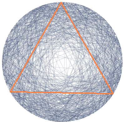
Inscribe an equilateral triangle in a circle. Randomly choose a line segment joining two points of this circle. What is the probability that this segment is longer than a side of the triangle?
This puzzle is called Bertrand's paradox, because different ways of solving it give different answers. To crack the paradox, you need to realize that it's meaningless to say you'll "randomly" choose something until you say more about how you're going to do it.
In other words, you can't compute the probability of an event until you pick a recipe for computing probabilities. Such a recipe is called a probability measure.
This applies to computing entropy, too! The formula for entropy clearly involves a probability distribution, even when our set of events is finite:
$$ S = - \sum_i p_i \ln(p_i) $$
But this formula conceals a fact that becomes obvious when our set of events is infinite. Now the sum becomes an integral:
$$ S = - \int_X p(x) \ln(p(x)) \, d x$$
And now it's clear that this formula makes no sense until we choose the measure $d x.$ On a finite set we have a god-given choice of measure, called counting measure. Integrals with respect to this are just sums. But in general we don't have such a god-given choice. And even for finite sets, working with counting measure is a choice: we are choosing to believe that in the absence of further evidence, all options are equally likely.
Taking this fact into account, it seems like we need two things to compute entropy: a probability distribution $p(x)$, and a measure $d x.$ That's on the right track. But an even better way to think of it is this:
$$ \displaystyle{ S = - \int_X \frac{p(x) dx}{dx} \ln \left(\frac{p(x) dx}{dx}\right) \, dx }$$
Now we see the entropy depends two measures: the probability measure $p(x) dx $ we care about, but also the measure $d x.$ Their ratio is important, but that's not enough: we also need one of these measures to do the integral. Above I used the measure $dx$ to do the integral, but we can also use $p(x) dx$ if we write
$$ \displaystyle{ S = - \int_X \ln \left(\frac{p(x) dx}{dx}\right) p(x) dx } $$
Either way, we are computing the entropy of one measure relative to another. So we might as well admit it, and talk about relative entropy.
The entropy of the measure $d \mu$ relative to the measure $d \nu$ is defined by:
$$ \begin{array}{ccl} S(d \mu, d \nu) &=& \displaystyle{ - \int_X \frac{d \mu(x) }{d \nu(x)} \ln \left(\frac{d \mu(x)}{ d\nu(x) }\right) d\nu(x) } \\ \; \\ &=& \displaystyle{ - \int_X \ln \left(\frac{d \mu(x)}{ d\nu(x) }\right) d\mu(x) } \end{array} $$
The second formula is simpler, but the first looks more like summing $-p \ln(p),$ so they're both useful.
Since we're taking entropy to be lack of information, we can also get rid of the minus sign and define relative information by
$$ \begin{array}{ccl} I(d \mu, d \nu) &=& \displaystyle{ \int_X \frac{d \mu(x) }{d \nu(x)} \ln \left(\frac{d \mu(x)}{ d\nu(x) }\right) d\nu(x) } \\ \; \\ &=& \displaystyle{ \int_X \ln \left(\frac{d \mu(x)}{ d\nu(x) }\right) d\mu(x) } \end{array} $$
If you thought something was randomly distributed according to the probability measure $d \nu,$ but then you you discover it's randomly distributed according to the probability measure $d \mu,$ how much information have you gained? The answer is $I(d\mu,d\nu).$
For more on relative entropy, read Part 6 of this series. I gave some examples illustrating how it works. Those should convince you that it's a useful concept.
Okay: now let's switch back to a more lowbrow approach. In the case of a finite set, we can revert to thinking of our two measures as probability distributions, and write the information gain as
$$ I(q,p) = \displaystyle{ \sum_i \ln \left(\frac{q_i}{p_i }\right) q_i} $$
If you want to sound like a Bayesian, call $p$ the prior probability distribution and $q$ the posterior probability distribution. Whatever you call them, $I(q,p)$ is the amount of information you get if you thought $p$ and someone tells you "no, $q$!"
We'll use this idea to think about how a population gains information about its environment as time goes by, thanks to natural selection. The rest of this post will be an exposition of Theorem 1 in this paper:
Harper says versions of this theorem ave previously appeared in work by Ethan Akin, and independently in work by Josef Hofbauer and Karl Sigmund. He also credits others here. An idea this good is rarely noticed by just one person.
So: consider $n$ different species of replicators. Let $P_i$ be the population of the $i$th species, and assume these populations change according to the replicator equation:
$$ \displaystyle{ \frac{d P_i}{d t} = f_i(P_1, \dots, P_n) \, P_i } $$
where each function $f_i$ depends smoothly on all the populations. And as usual, we let
$$ \displaystyle{ p_i = \frac{P_i}{\sum_j P_j} } $$
be the fraction of replicators in the $i$th species.
Let's study the relative information $I(q,p)$ where $q$ is some fixed probability distribution. We'll see something great happens when $q$ is a stable equilibrium solution of the replicator equation. In this case, the relative information can never increase! It can only decrease or stay constant.
We'll think about what all this means later. First, let's see that it's true! Remember,
$$ \begin{array}{ccl} I(q,p) &=& \displaystyle{ \sum_i \ln \left(\frac{q_i}{ p_i }\right) q_i } \\ \; \\ &=& \displaystyle{ \sum_i \Big(\ln(q_i) - \ln(p_i) \Big) q_i } \end{array}$$
and only $p_i$ depends on time, not $q_i$, so
$$ \begin{array}{ccl} \displaystyle{ \frac{d}{dt} I(q,p)} &=& \displaystyle{ - \frac{d}{dt} \sum_i \ln(p_i) q_i }\\ \; \\ &=& \displaystyle{ - \sum_i \frac{\dot{p}_i}{p_i} \, q_i } \end{array} $$
where $\dot{p}_i$ is the rate of change of the probability $p_i.$ We saw a nice formula for this in Part 9:
$$ \displaystyle{ \dot{p}_i = \Big( f_i(P) - \langle f(P) \rangle \Big) \, p_i }$$
where
$$ f_i(P) = f_i(P_1, \dots, P_n) $$
and
$$ \displaystyle{ \langle f(P) \rangle = \sum_i f_i(P) p_i } $$
is the mean fitness of the species. So, we get
$$ \displaystyle{ \frac{d}{dt} I(q,p) } = \displaystyle{ - \sum_i \Big( f_i(P) - \langle f(P) \rangle \Big) \, q_i } $$
Nice, but we can fiddle with this expression to get something more enlightening. Remember, the numbers $q_i$ sum to one. So:
$$ \begin{array}{ccl} \displaystyle{ \frac{d}{dt} I(q,p) } &=& \displaystyle{ \langle f(P) \rangle - \sum_i f_i(P) q_i } \\ \; \\ &=& \displaystyle{ \sum_i f_i(P) (p_i - q_i) } \end{array} $$
where in the last step I used the definition of the mean fitness. This result looks even cuter if we treat the numbers $f_i(P)$ as the components of a vector $f(P),$ and similarly for the numbers $p_i$ and $q_i.$ Then we can use the dot product of vectors to say
$$ \displaystyle{ \frac{d}{dt} I(q,p) = f(P) \cdot (p - q) }$$
So, the relative information $I(q,p)$ will always decrease if
$$ f(P) \cdot (p - q) \le 0$$
for all choices of the population $P$.
And now something really nice happens: this is also the condition for $q$ to be an evolutionarily stable state. This concept goes back to John Maynard Smith, the founder of evolutionary game theory. In 1982 he wrote:
A population is said to be in an evolutionarily stable state if its genetic composition is restored by selection after a disturbance, provided the disturbance is not too large.
I will explain the math next time—I need to straighten out some things in my mind first. But the basic idea is compelling: an evolutionarily stable state is like a situation where our replicators 'know all there is to know' about the environment and each other. In any other state, the population has 'something left to learn'—and the amount left to learn is the relative information we've been talking about! But as time goes on, the information still left to learn decreases!
Note: in the real world, nature has never found an evolutionarily stable state... except sometimes approximately, on sufficiently short time scales, in sufficiently small regions. So we are still talking about an idealization of reality! But that's okay, as long as we know it.
You can read a discussion of this article on Azimuth, and make your own comments or ask questions there!
|
|
|
|