

|
|
|
|
Now I'll tell you a bit about what it actually says!
Remember the story so far: we've got a physical system that's in a state of maximum entropy. I didn't emphasize this yet, but that happens whenever our system is in thermodynamic equilibrium. An example would be a box of gas inside a piston. Suppose you choose any number for the energy of the gas and any number for its volume. Then there's a unique state of the gas that maximizes its entropy, given the constraint that on average, its energy and volume have the values you've chosen. And this describes what the gas will be like in equilibrium!
Remember, by 'state' I mean mixed state: it's a probabilistic description. And I say the energy and volume have chosen values on average because there will be random fluctuations. Indeed, if you look carefully at the head of the piston, you'll see it quivering: the volume of the gas only equals the volume you've specified on average. Same for the energy.
More generally: imagine picking any list of numbers, and finding the maximum entropy state where some chosen observables have these numbers as their average values. Then there will be fluctuations in the values of these observables — thermal fluctuations, but also possibly quantum fluctuations. So, you'll get a probability distribution on the space of possible values of your chosen observables. You should visualize this probability distribution as a little fuzzy cloud centered at the average value!
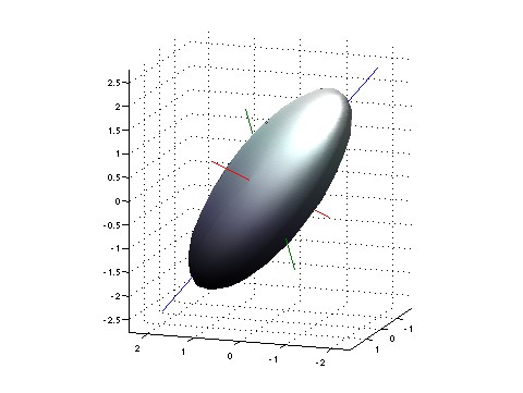
To a first approximation, this cloud will be shaped like a little ellipsoid. And if you can pick the average value of your observables to be whatever you'll like, you'll get lots of little ellipsoids this way, one centered at each point. And the cool idea is to imagine the space of possible values of your observables as having a weirdly warped geometry, such that relative to this geometry, these ellipsoids are actually spheres.
This weirdly warped geometry is an example of an 'information geometry': a geometry that's defined using the concept of information. This shouldn't be surprising: after all, we're talking about maximum entropy, and entropy is related to information. But I want to gradually make this idea more precise. Bring on the math!
We've got a bunch of observables $ X_1, \dots , X_n$, and we're assuming that for any list of numbers $ x_1, \dots , x_n$, the system has a unique maximal-entropy state $ \rho$ for which the expected value of the observable $ X_i$ is $ x_i$:
$$ \langle X_i \rangle = x_i $$This state $ \rho$ is called the Gibbs state and I told you how to find it when it exists. In fact it may not exist for every list of numbers $ x_1, \dots , x_n$, but we'll be perfectly happy if it does for all choices of
$$ x = (x_1, \dots, x_n) $$lying in some open subset of $ \mathbb{R}^n$
By the way, I should really call this Gibbs state $ \rho(x)$ or something to indicate how it depends on $ x$, but I won't usually do that. I expect some intelligence on your part!
Now at each point $ x$ we can define a covariance matrix
$$ \langle (X_i - \langle X_i \rangle) (X_j - \langle X_j \rangle) \rangle $$If we take its real part, we get a symmetric matrix:
$$ g_{ij} = \mathrm{Re} \langle (X_i - \langle X_i \rangle) (X_j - \langle X_j \rangle) \rangle $$It's also nonnegative — that's easy to see, since the variance of a probability distribution can't be negative. When we're lucky this matrix will be positive definite. When we're even luckier, it will depend smoothly on $ x$. In this case, $ g_{ij}$ will define a Riemannian metric on our open set.
So far this is all review of last time. Sorry: I seem to have reached the age where I can't say anything interesting without warming up for about 15 minutes first. It's like when my mom tells me about an exciting event that happened to her: she starts by saying "Well, I woke up, and it was cloudy out..."
But now I want to give you an explicit formula for the metric $ g_{ij}$, and then rewrite it in a way that'll work even when the state $ \rho$ is not a maximal-entropy state. And this formula will then be the general definition of the 'Fisher information metric' (if we're doing classical mechanics), or a quantum version thereof (if we're doing quantum mechanics).
Crooks does the classical case — so let's do the quantum case, okay? Last time I claimed that in the quantum case, our maximum-entropy state is the Gibbs state
$$ \rho = \frac{1}{Z} e^{-\lambda^i X_i}$$where $ \lambda^i$ are the 'conjugate variables' of the observables $ X_i$, we're using the Einstein summation convention to sum over repeated indices that show up once upstairs and once downstairs, and $ Z$ is the partition function
$$ Z = \mathrm{tr} (e^{-\lambda^i X_i})$$(To be honest: last time I wrote the indices on the conjugate variables $ \lambda^i$ as subscripts rather than superscripts, because I didn't want some poor schlep out there to think that $ \lambda^1, \dots , \lambda^n$ were the powers of some number $ \lambda$. But now I'm assuming you're all grown up and ready to juggle indices! We're doing Riemannian geometry, after all.)
Also last time I claimed that it's tremendously fun and enlightening to take the derivative of the logarithm of $ Z$. The reason is that it gives you the mean values of your observables:
$$ \langle X_i \rangle = - \frac{\partial}{\partial \lambda^i} \ln Z $$But now let's take the derivative of the logarithm of $ \rho$. Remember, $ \rho$ is an operator — in fact a density matrix. But we can take its logarithm as explained last time, and the usual rules apply, so starting from
$$ \rho = \frac{1}{Z} e^{-\lambda^i X_i}$$we get
$$ \mathrm{ln}\, \rho = - \lambda^i X_i - \mathrm{ln} \,Z $$Next, let's differentiate both sides with respect to $ \lambda^i$. Why? Well, from what I just said, you should be itching to differentiate $ \mathrm{ln}\, Z$. So let's give in to that temptation:
$$ \frac{\partial }{\partial \lambda^i} \mathrm{ln} \rho = -X_i + \langle X_i \rangle $$Hey! Now we've got a formula for the 'fluctuation' of the observable $ X_i$ — that is, how much it differs from its mean value:
$$ X_i - \langle X_i \rangle = - \frac{\partial \mathrm{ln} \rho }{\partial \lambda^i}$$This is incredibly cool! I should have learned this formula decades ago, but somehow I just bumped into it now. I knew of course that $ \mathrm{ln} \, \rho$ shows up in the formula for the entropy:
$$ S(\rho) = \mathrm{tr} ( \rho \; \mathrm{ln} \, \rho) $$But I never had the brains to think about $ \mathrm{ln}\, \rho$ all by itself. So I'm really excited to discover that it's an interesting entity in its own right — and fun to differentiate, just like $ \mathrm{ln}\, Z$.
Now we get our cool formula for $ g_{ij}$. Remember, it's defined by
$$ g_{ij} = \mathrm{Re} \langle (X_i - \langle X_i \rangle) (X_j - \langle X_j \rangle) \rangle $$But now that we know
$$ X_i - \langle X_i \rangle = -\frac{\partial \mathrm{ln} \rho }{\partial \lambda^i}$$we get the formula we were looking for:
$$ g_{ij} = \mathrm{Re} \left\langle \frac{\partial \mathrm{ln} \rho }{\partial \lambda^i} \; \frac{\partial \mathrm{ln} \rho }{\partial \lambda^j} \right\rangle $$Beautiful, eh? And of course the expected value of any observable $ A$ in the state $ \rho$ is
$$ \langle A \rangle = \mathrm{tr}(\rho A)$$so we can also write the covariance matrix like this:
$$ g_{ij} = \mathrm{Re}\, \mathrm{tr}\left(\rho \; \frac{\partial \mathrm{ln} \rho }{\partial \lambda^i} \; \frac{\partial \mathrm{ln} \rho }{\partial \lambda^j} \right) $$Lo and behold! This formula makes sense whenever $ \rho$ is any density matrix depending smoothly on some parameters $ \lambda^i$. We don't need it to be a Gibbs state! So, we can work more generally.
Indeed, whenever we have any smooth function from a manifold to the space of density matrices for some Hilbert space, we can define $ g_{ij}$ by the above formula! And when it's positive definite, we get a Riemannian metric on our manifold: the Bures information metric.
The classical analogue is the somewhat more well-known 'Fisher information metric'. When we go from quantum to classical, operators become functions and traces become integrals. There's nothing complex anymore, so taking the real part becomes unnecessary. So the Fisher information metric looks like this:
$$ g_{ij} = \int_\Omega p(\omega) \; \frac{\partial \mathrm{ln} p(\omega) }{\partial \lambda^i} \; \frac{\partial \mathrm{ln} p(\omega) }{\partial \lambda^j} \; d \omega $$Here I'm assuming we've got a smooth function $ p$ from some manifold $ M$ to the space of probability distributions on some measure space $ (\Omega, d\omega)$. Working in local coordinates $ \lambda^i$ on our manifold $ M$, the above formula defines a Riemannian metric on $ M$, at least when $ g_{ij}$ is positive definite. And that's the Fisher information metric!
Crooks says more: he describes an experiment that would let you measure the length of a path with respect to the Fisher information metric — at least in the case where the state $ \rho(x)$ is the Gibbs state with $ \langle X_i \rangle = x_i$. And that explains why he calls it 'thermodynamic length'.
There's a lot more to say about this, and also about another question: What use is the Fisher information metric in the general case where the states $ \rho(x)$ aren't Gibbs states?
But it's dinnertime, so I'll stop here.
You can read a discussion of this article on Azimuth, and make your own comments or ask questions there!
|
|
|
|