

|
|
|
|
I think it will help to do an example. The harmonic oscillator is a trusty workhorse throughout physics, so let's do that.
So: suppose you have a rock hanging on a spring, and it can bounce up and down. Suppose it's in thermal equilibrium with its environment. It will wiggle up and down ever so slightly, thanks to thermal fluctuations. The hotter it is, the more it wiggles. These vibrations are random, so its position and momentum at any given moment can be treated as random variables.
If we take quantum mechanics into account, there's an extra source of randomness: quantum fluctuations. Now there will be fluctuations even at zero temperature. Ultimately this is due to the uncertainty principle. Indeed, if you know the position for sure, you can't know the momentum at all!
Let's see how the position, momentum and energy of our rock will fluctuate given that we know all three of these quantities on average. The fluctuations will form a little fuzzy blob, roughly ellipsoidal in shape, in the 3-dimensional space whose coordinates are position, momentum and energy:
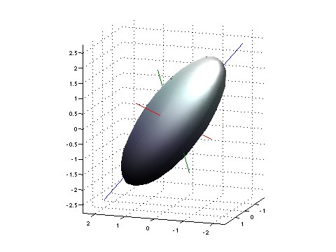
Yeah, I know you're sick of this picture, but this time it's for real: I want to calculate what this ellipsoid actually looks like! I'm not promising I'll do it — I may get stuck, or bored — but at least I'll try.
Before I start the calculation, let's guess the answer. A harmonic oscillator has a position $q$ and momentum $p$, and its energy is
$$ H = \frac{1}{2}(q^2 + p^2)$$Here I'm working in units where lots of things equal 1, to keep things simple.
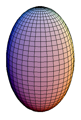
You'll notice that this energy has rotational symmetry in the position-momentum plane. This is ultimately what makes the harmonic oscillator such a beloved physical system. So, we might naively guess that our little ellipsoid will have rotational symmetry as well, like this:
or this:
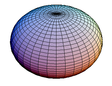
Here I'm using the $x$ and $y$ coordinates for position and momentum, while the $z$ coordinate stands for energy. So in these examples the position and momentum fluctuations are the same size, while the energy fluctuations, drawn in the vertical direction, might be bigger or smaller.
Unfortunately, this guess really is naive. After all, there are lots of these ellipsoids, one centered at each point in position-momentum-energy space. Remember the rules of the game! You give me any point in this space. I take the coordinates of this point as the mean values of position, momentum and energy, and I find the maximum-entropy state with these mean values. Then I work out the fluctuations in this state, and draw them as an ellipsoid.
If you pick a point where position and momentum have mean value zero, you haven't broken the rotational symmetry of the problem. So, my ellipsoid must be rotationally symmetric. But if you pick some other mean value for position and momentum, all bets are off!
Fortunately, this naive guess is actually right: all the ellipsoids are rotationally symmetric — even the ones centered at nonzero values of position and momentum! We'll see why soon. And if you've been following this series of posts, you'll know what this implies: the "Fisher information metric" $g$ on position-momentum-energy space has rotational symmetry about any vertical axis. (Again, I'm using the vertical direction for energy.) So, if we slice this space with any horizontal plane, the metric on this plane must be the plane's usual metric times a constant:
$$ g = \mathrm{constant} \, (dq^2 + dp^2) $$Why? Because only the usual metric on the plane, or any multiple of it, has ordinary rotations around every point as symmetries.
So, roughly speaking, we're recovering the 'obvious' geometry of the position-momentum plane from the Fisher information metric. We're recovering 'ordinary' geometry from information geometry!
But this should not be terribly surprising, since we used the harmonic oscillator Hamiltonian
$$ H = \frac{1}{2}(q^2 + p^2)$$as an input to our game. It's mainly just a confirmation that things are working as we'd hope.
There's more, though. Last time I realized that because observables in quantum mechanics don't commute, the Fisher information metric has a curious skew-symmetric partner called $\omega$. So, we should also study this in our example. And when we do, we'll see that restricted to any horizontal plane in position-momentum-energy space, we get
$$ \omega = \mathrm{constant} \, (dq \, dp - dp \, dq)$$This looks like a mutant version of the Fisher information metric
$$ g = \mathrm{constant} \, (dq^2 + dp^2) $$and if you know your geometry, you'll know it's the usual 'symplectic structure' on the position-energy plane — at least, times some constant.
All this is very reminiscent of Öttinger's work on dissipative mechanics. But we'll also see something else: while the constant in $g$ depends on the energy — that is, on which horizontal plane we take — the constant in $\omega$ does not!
Why? It's perfectly sensible. The metric $g$ on our horizontal plane keeps track of fluctuations in position and momentum. Thermal fluctuations get bigger when it's hotter — and to boost the average energy of our oscillator, we must heat it up. So, as we increase the energy, moving our horizontal plane further up in position-momentum-energy space, the metric on the plane gets bigger! In other words, our ellipsoids get a fat cross-section at high energies.
On the other hand, the symplectic structure $\omega$ arises from the fact that position $q$ and momentum $p$ don't commute in quantum mechanics. They obey Heisenberg's 'canonical commutation relation':
$$ q p - p q = i $$This relation doesn't involve energy, so $\omega$ will be the same on every horizontal plane. And it turns out this relation implies
$$ \omega = \mathrm{constant} \, (dq \, dp - dp \, dq)$$for some constant we'll compute later.
Okay, that's the basic idea. Now let's actually do some computations. For starters, let's see why all our ellipsoids have rotational symmetry!
To do this, we need to understand a bit about the mixed state $\rho$ that maximizes entropy given certain mean values of position, momentum and energy. So, let's choose the numbers we want for these mean values (also known as 'expected values' or 'expectation values'):
$$ \langle H \rangle = E $$ $$ \langle q \rangle = q_0$$ $$ \langle p \rangle = p_0$$I hope this isn't too confusing: $H, p, q$ are our observables which are operators, while $E, p_0, q_0$ are the mean values we have chosen for them. The state $\rho$ depends on $E, p_0$ and $q_0$.
We're doing quantum mechanics, so position $q$ and momentum $p$ are both self-adjoint operators on the Hilbert space $L^2(\mathbb{R})$:
$$ (q\psi)(x) = x \psi(x) $$ $$ (p\psi)(x) = - i \frac{d \psi}{dx}(x)$$Indeed all our observables, including the Hamiltonian
$$ H = \frac{1}{2} (p^2 + q^2) $$are self-adjoint operators on this Hilbert space, and the state $\rho$ is a density matrix on this space, meaning a positive self-adjoint operator with trace 1.
Now: how do we compute $\rho$? It's a Lagrange multiplier problem: maximizing some function given some constraints. And it's well-known that when you solve this problem, you get
$$ \rho = \frac{1}{Z} e^{-(\lambda^1 q + \lambda^2 p + \lambda^3 H)} $$where $\lambda^1, \lambda^2, \lambda^3$ are three numbers we yet have to find, and $Z$ is a normalizing factor called the partition function:
$$ Z = \mathrm{tr} (e^{-(\lambda^1 q + \lambda^2 p + \lambda^3 H)} )$$Now let's look at a special case. If we choose $\lambda^1 = \lambda^2 = 0$, we're back a simpler and more famous problem, namely maximizing entropy subject to a constraint only on energy! The solution is then
$$ \rho = \frac{1}{Z} e^{-\beta H} , \qquad Z = \mathrm{tr} (e^{- \beta H} )$$Here I'm using the letter $\beta$ instead of $\lambda^3$ because this is traditional. This quantity has an important physical meaning! It's the reciprocal of temperature in units where Boltzmann's constant is 1.
Anyway, back to our special case! In this special case it's easy to explicitly calculate $\rho$ and $Z$. Indeed, people have known how ever since Planck put the 'quantum' in quantum mechanics! He figured out how black-body radiation works. A box of hot radiation is just a big bunch of harmonic oscillators in thermal equilibrium. You can work out its partition function by multiplying the partition function of each one.
So, it would be great to reduce our general problem to this special case. To do this, let's rewrite
$$ Z = \mathrm{tr} (e^{-(\lambda^1 q + \lambda^2 p + \lambda^3 H)} )$$in terms of some new variables, like this:
$$ \rho = \frac{1}{Z} e^{-\beta(H - f q - g p)} $$where now
$$ Z = \mathrm{tr} (e^{-\beta(H - f q - g p)} )$$Think about it! Now our problem is just like an oscillator with a modified Hamiltonian
$$ H' = H - f q - g p$$What does this mean, physically? Well, if you push on something with a force $f$, its potential energy will pick up a term $- f q$. So, the first two terms are just the Hamiltonian for a harmonic oscillator with an extra force pushing on it!
I don't know a nice interpretation for the $- g p$ term. We could say that besides the extra force equal to $f$, we also have an extra 'gorce' equal to $g$. I don't know what that means. Luckily, I don't need to! Mathematically, our whole problem is invariant under rotations in the position-momentum plane, so whatever works for $q$ must also work for $p$.
Now here's the cool part. We can complete the square:
$$ \begin{aligned} H' & = \frac{1}{2} (q^2 + p^2) - f q - g p \\ &= \frac{1}{2}(q^2 - 2 q f + f^2) + \frac{1}{2}(p^2 - 2 q g + g^2) - \frac{1}{2}(g^2 + f^2) \\ &= \frac{1}{2}((q - f)^2 + (p - g)^2) - \frac{1}{2}(g^2 + f^2) \end{aligned}$$so if we define 'translated' position and momentum operators:
$$ q' = q - f, \qquad p' = p - g $$we have
$$ H' = \frac{1}{2}({q'}^2 + {p'}^2) - \frac{1}{2}(g^2 + f^2) $$So: apart from a constant, $H'$ is just the harmonic oscillator Hamiltonian in terms of 'translated' position and momentum operators!
In other words: we're studying a strange variant of the harmonic oscillator, where we are pushing on it with an extra force and also an extra 'gorce'. But this strange variant is exactly the same as the usual harmonic oscillator, except that we're working in translated coordinates on position-momentum space, and subtracting a constant from the Hamiltonian.
These are pretty minor differences. So, we've succeeded in reducing our problem to the problem of a harmonic oscillator in thermal equilibrium at some temperature!
This makes it easy to calculate
$$ Z = \mathrm{tr} (e^{-\beta(H - f q - g p)} ) = \mathrm{tr}(e^{-\beta H'})$$By our formula for $H'$, this is just
$$ Z = e^{\frac{1}{2}(g^2 + f^2)} \; \mathrm{tr} (e^{-\frac{1}{2}({q'}^2 + {p'}^2)})$$And the second factor here equals the partition function for the good old harmonic oscillator:
$$ Z = e^{\frac{1}{2}(g^2 + f^2)} \; \mathrm{tr} (e^{-\beta H})$$So now we're back to a textbook problem. The eigenvalues of the harmonic oscillator Hamiltonian are
$$ n + \frac{1}{2}$$where
$$ n = 0,1,2,3, \dots$$So, the eigenvalues of $e^{-\beta H}$ are are just
$$ e^{-\beta(n + \frac{1}{2})} $$and to take the trace of this operator, we sum up these eigenvalues:
$$ \mathrm{tr}(e^{-\beta H}) = \sum_{n = 0}^\infty e^{-\beta (n + \frac{1}{2})} = \frac{e^{-\beta/2}}{1 - e^{-\beta}} $$So:
$$ Z = e^{\frac{1}{2}(g^2 + f^2)} \; \frac{e^{-\beta/2}}{1 - e^{-\beta}} $$We can now compute the Fisher information metric using this formula:
$$ g_{ij} = \frac{\partial^2}{\partial \lambda^i \partial \lambda^j} \ln Z$$if we remember how our new variables are related to the $\lambda^i$:
$$ \lambda^1 = \beta f , \qquad \lambda^2 = \beta g, \qquad \lambda^3 = \beta$$It's just calculus! But I'm feeling a bit tired, so I'll leave this pleasure to you.
For now, I'd rather go back to our basic intuition about how the Fisher information metric describes fluctuations of observables. Mathematically, this means it's the real part of the covariance matrix
$$ g_{ij} = \mathrm{Re} \langle \, (X_i - \langle X_i \rangle) \, (X_j - \langle X_j \rangle) \, \rangle $$where for us
$$ X_1 = q, \qquad X_2 = p, \qquad X_3 = E $$Here we are taking expected values using the mixed state $\rho$. We've seen this mixed state is just like the maximum-entropy state of a harmonic oscillator at fixed temperature — except for two caveats: we're working in translated coordinates on position-momentum space, and subtracting a constant from the Hamiltonian. But neither of these two caveats affects the fluctuations $(X_i - \langle X_i \rangle)$ or the covariance matrix.
So, as indeed we've already seen, $g_{ij}$ has rotational symmetry in the 1-2 plane. Thus, we'll completely know it once we know $g_{11} = g_{22}$ and $g_{33}$; the other components are zero for symmetry reasons. $g_{11}$ will equal the variance of position for a harmonic oscillator at a given temperature, while $g_{33}$ will equal the variance of its energy. We can work these out or look them up.
I won't do that now: I'm after insight, not formulas. For physical reasons, it's obvious that $g_{11}$ must diminish with diminishing energy — but not go to zero. Why? Well, as the temperature approaches zero, a harmonic oscillator in thermal equilibrium approaches its state of least energy: the so-called 'ground state'. In its ground state, the standard deviations of position and momentum are as small as allowed by the Heisenberg uncertainty principle:
$$ \Delta p \Delta q \ge \frac{1}{2}$$and they're equal, so
$$ g_{11} = (\Delta q)^2 = \frac{1}{2}$.That's enough about the metric. Now, what about the metric's skew-symmetric partner? This is:
$$ \omega_{ij} = \mathrm{Im} \langle \, (X_i - \langle X_i \rangle) \, (X_j - \langle X_j \rangle) \, \rangle $$Last time we saw that $\omega$ is all about expected values of commutators:
$$ \omega_{ij} = \frac{1}{2i} \langle [X_i, X_j] \rangle$$and this makes it easy to compute. For example,
$$ [X_1, X_2] = q p - p q = i$$so
$$ \omega_{12} = \frac{1}{2} $ Of course $$ \omega_{11} = \omega_{22} = 0$$by skew-symmetry, so we know the restriction of $\omega$ to any horizontal plane. We can also work out other components, like $\omega_{13}$, but I don't want to. I'd rather just state this:
Summary: Restricted to any horizontal plane in the position-momentum-energy space, the Fisher information metric for the harmonic oscillator is $$ g = \mathrm{constant} (dq_0^2 + dp_0^2) $$with a constant depending on the temperature, equalling $\frac{1}{2}$ in the zero-temperature limit, and increasing as the temperature rises. Restricted to the same plane, the Fisher information metric's skew-symmetric partner is
$$ \omega = \frac{1}{2} dq_0 \wedge dp_0 $$
(Remember, the mean values $q_0, p_0, E_0$ are the coordinates on position-momentum-energy space. We could also use coordinates $f, g, \beta$ or $f, g$ and temperature. In the chatty intro to this article you saw formulas like those above but without the subscripts; that's before I got serious about using $q$ and $p$ to mean operators.)
And now for the moral. Actually I have two: a physics moral and a math moral.
First, what is the physical meaning of $g$ or $\omega$ when restricted to a plane of constant $E_0$, or if you prefer, a plane of constant temperature?
Physics Moral: Restricted to a constant-temperature plane, $g$ is the covariance matrix for our observables. It is temperature-dependent. In the zero-temperature limit, the thermal fluctuations go away and $g$ depends only on quantum fluctuations in the ground state. On the other hand, $\omega$ restricted to a constant-temperature plane describes Heisenberg uncertainty relations for noncommuting observables. In our example, it is temperature-independent.
Second, what does this have to do with Kähler geometry? Remember, the complex plane has a complex-valued metric on it, called a Kähler structure. Its real part is a Riemannian metric, and its imaginary part is a symplectic structure. We can think of the the complex plane as the position-momentum plane for a point particle. Then the symplectic structure is the basic ingredient needed for Hamiltonian mechanics, while the Riemannian structure is the basic ingredient needed for the harmonic oscillator Hamiltonian.
Math Moral: In the example we considered, $\omega$ restricted to a constant-temperature plane is equal to $\frac{1}{2}$ the usual symplectic structure on the complex plane. On the other hand, $g$ restricted to a constant-temperature plane is a multiple of the usual Riemannian metric on the complex plane — but this multiple is $\frac{1}{2}$ only when the temperature is zero! So, only at temperature zero are $g$ and $\omega$ the real and imaginary parts of a Kähler structure.
It will be interesting to see how much of this stuff is true more generally. The harmonic oscillator is much nicer than your average physical system, so it can be misleading, but I think some of the morals we've seen here can be generalized.
Some other time I may so more about how all this is related to Öttinger's formalism, but the quick point is that he too has mixed states, and a symmetric $g$, and a skew-symmetric $\omega$. So it's nice to see if they match up in an example.
Finally, two footnotes on terminology:
β: In fact, this quantity $\beta = 1/kT$ is so important it deserves a better name than 'reciprocal of temperature'. How about 'coolness'? An important lesson from statistical mechanics is that coolness is more fundamental than temperature. This makes some facts more plausible. For example, if you say "you can never reach absolute zero," it sounds very odd, since you can get as close as you like, and it's even possible to get negative temperatures — but temperature zero remains tantalizingly out of reach. But "you can never attain infinite coolness" — now that makes sense.
Gorce: I apologize to Richard Feynman for stealing the word 'gorce' and using it a different way. Does anyone have a good intuition for what's going on when you apply my sort of 'gorce' to a point particle? You need to think about velocity-dependent potentials, of that I'm sure. In the presence of a velocity-dependent potential, momentum is not just mass times velocity. Which is good: if it were, we could never have a system where the mean value of both $q$ and $p$ stayed constant over time!
You can read a discussion of this article on Azimuth, and make your own comments or ask questions there!
|
|
|
|