This was a very difficult chapter for me to teach, at least near the end, because it covered some central topics in category theory at a very rapid pace. It was hard to resist going into more detail... but I felt that this chapter was more intimidating than the previous ones, and that more detail might make things even worse!
For example, I said that an adjunction is a pair of functors \\(F: \mathcal{A} \to \mathcal{B}\\) and \\(G: \mathcal{B} \to \mathcal{A}\\) equipped with a natural isomorphism
\[ \alpha : \mathcal{B}(F(-),-) \to \mathcal{A}(-,G(-)). \]
I told you what a natural isomorphism is, and we saw what this particular isomorphism is like in some examples... but I didn't really say what benefit we get out of it being _natural_.
We would see this if we discussed how adjunctions give [monads](https://en.wikipedia.org/wiki/Monad_(category_theory)), but the textbook doesn't discuss monads at all! I hear hundreds of Haskell programmers groaning in dismay... but presumably this decision was made because monads are already covered by plenty of more traditional textbooks.
Another thing that pains me is this: I don't think I managed to give enough examples to fully explain the sense in which left adjoints are 'liberal' or 'generous' while right adjoints are 'conservative' or 'cautious'.
I also didn't explain _why_, whenever you have a functor \\(G : \mathcal{D} \to \mathcal{C}\\), the functor
\[ \text{composition with } G : \mathbf{Set}^\mathcal{C} \to \mathbf{Set}^{\mathcal{D}} \]
has both a left adjoint
\[ \text{Lan}_G : \mathbf{Set}^{\mathcal{D}} \to \mathbf{Set}^{\mathcal{C}} \]
called **left Kan extenson along \\(G\\)**, and a right adjoint
\[ \text{Ran}_G : \mathbf{Set}^{\mathcal{D}} \to \mathbf{Set}^{\mathcal{C}} \]
called **right Kan extension along \\(G\\)**.
Our textbook makes a good stab at this in one case: the case where \\(\mathcal{C}\\) is \\(\mathbf{1}\\), the category with one object and one morphism. There exists a unique functor from any category \\(\mathcal{D}\\) to \\(\mathbf{1}\\), usually denoted
\[ ! : \mathcal{D} \to \mathbf{1} \]
Right Kan extension along \\(!\\) is a functor
\[ \text{Ran}_! : \mathbf{Set}^{\mathcal{D}} \to \mathbf{Set}^{\mathbf{1}} \]
but since \\(\mathbf{Set}^{\mathbf{1}}\\) is isomorphic to \\(\mathbf{Set}\\), we can think of it as a functor
\[ \lim_{\mathcal{D}} : \mathbf{Set}^{\mathcal{D}} \to \mathbf{Set} \]
I'm using this funny notation because that's what this functor is usually called: in particular, given an object \\(F\\) in \\(\mathbf{Set}^{\mathcal{D}}\\), meaning a functor \\(F : \mathcal{D} \to \mathbf{Set}\\), we get a set called its **limit**,
\[ \displaystyle{\lim_{\mathcal{D}} F}. \]
And Theorem 3.79 in this book says how to compute it!
Similarly, the left Kan extension along \\(!\\) is called a **colimit**. [Limits](https://en.wikipedia.org/wiki/Limit_(category_theory)) and [colimits](https://en.wikipedia.org/wiki/Limit_(category_theory)#Colimits) are very important in category theory - but again, they're covered in great detail in all the standard textbooks, so Fong and Spivak didn't feel the need to dwell on them.
So much to explain, so little time!  Please ask questions if you want to know more about anything. As for my lectures, I must now move on to Chapter 4. I'll just leave you with a few puzzles:
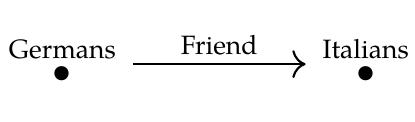
**Puzzle 166.** Let \\(\mathcal{D}\\) be the free category on this graph:
Please ask questions if you want to know more about anything. As for my lectures, I must now move on to Chapter 4. I'll just leave you with a few puzzles:
**Puzzle 166.** Let \\(\mathcal{D}\\) be the free category on this graph:
 and let \\(\mathbf{1}\\) be the free category on this graph:
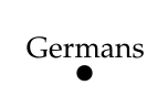 (This is just a German-centered way of thinking about the category with one object and one morphism.) Take a database \\(F: \mathbf{1} \to \mathbf{Set}\\), for example this:
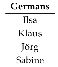 What is the database \\( F \circ ! :\mathcal{D} \to \mathbf{Set}\\)?
**Puzzle 167.** Next, take a database \\(H: \mathcal{C} \to \mathbf{Set}\\), for example this:
What is the database \\( F \circ ! :\mathcal{D} \to \mathbf{Set}\\)?
**Puzzle 167.** Next, take a database \\(H: \mathcal{C} \to \mathbf{Set}\\), for example this:
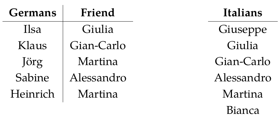 What is the database \\(\mathrm{Ran}\_! : \mathbf{1} \to \mathbf{Set}\\)? What is the database \\(\mathrm{Lan}\_! : \mathbf{1} \to \mathbf{Set}\\)?
**Puzzle 168.** Suppose \\(F\\) is a left adjoint of \\(G\\), as above. If \\(a \in \mathrm{Ob}(\mathcal{A})\\) and \\(b \in \mathrm{Ob}(\mathcal{B})\\) we get a bijection
\[ \alpha_{a,b} : \mathcal{B}(F(a),b) \to \mathcal{A}(a,G(b)). \]
Similarly, if \\(a' \in \mathrm{Ob}(\mathcal{A})\\) and \\(b' \in \mathrm{Ob}(\mathcal{B})\\) we get a bijection
\[ \alpha_{a',b'} : \mathcal{B}(F(a'),b') \to \mathcal{A}(a',G(b')). \]
Show that if \\(f: a' \to a\\) and \\(g: b \to b'\\) we get a commutative square
\[
\begin{matrix}
& & \alpha_{a,b} & & \\\\
& \mathcal{B}(F(a),b) & \rightarrow & \mathcal{A}(a,G(b)) &\\\\
\mathcal{B}(F(f),g) & \downarrow & & \downarrow & \mathcal{A}(f,G(g)) \\\\
& \mathcal{B}(F(a'),b') & \rightarrow & \mathcal{A}(a',G(b')) &\\\\
& & \alpha_{a',b'} & & \\\\
\end{matrix}
\]
To see what this means concretely, take a guy \\(h \in \mathcal{B}(F(a),b) \\), meaning a morphism \\(h : F(a) \to b\\), and send it around the square both ways: down and then across, or across and then down. You get two morphisms from \\( a' \\) to \\(G(b')\\); what are they? Since the square commutes these must be equal.
**[To read other lectures go here.](http://www.azimuthproject.org/azimuth/show/Applied+Category+Theory#Chapter_3)**
What is the database \\(\mathrm{Ran}\_! : \mathbf{1} \to \mathbf{Set}\\)? What is the database \\(\mathrm{Lan}\_! : \mathbf{1} \to \mathbf{Set}\\)?
**Puzzle 168.** Suppose \\(F\\) is a left adjoint of \\(G\\), as above. If \\(a \in \mathrm{Ob}(\mathcal{A})\\) and \\(b \in \mathrm{Ob}(\mathcal{B})\\) we get a bijection
\[ \alpha_{a,b} : \mathcal{B}(F(a),b) \to \mathcal{A}(a,G(b)). \]
Similarly, if \\(a' \in \mathrm{Ob}(\mathcal{A})\\) and \\(b' \in \mathrm{Ob}(\mathcal{B})\\) we get a bijection
\[ \alpha_{a',b'} : \mathcal{B}(F(a'),b') \to \mathcal{A}(a',G(b')). \]
Show that if \\(f: a' \to a\\) and \\(g: b \to b'\\) we get a commutative square
\[
\begin{matrix}
& & \alpha_{a,b} & & \\\\
& \mathcal{B}(F(a),b) & \rightarrow & \mathcal{A}(a,G(b)) &\\\\
\mathcal{B}(F(f),g) & \downarrow & & \downarrow & \mathcal{A}(f,G(g)) \\\\
& \mathcal{B}(F(a'),b') & \rightarrow & \mathcal{A}(a',G(b')) &\\\\
& & \alpha_{a',b'} & & \\\\
\end{matrix}
\]
To see what this means concretely, take a guy \\(h \in \mathcal{B}(F(a),b) \\), meaning a morphism \\(h : F(a) \to b\\), and send it around the square both ways: down and then across, or across and then down. You get two morphisms from \\( a' \\) to \\(G(b')\\); what are they? Since the square commutes these must be equal.
**[To read other lectures go here.](http://www.azimuthproject.org/azimuth/show/Applied+Category+Theory#Chapter_3)**