

|
|
|
|
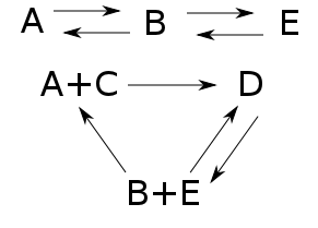
Recently we've been talking about 'reaction networks', like this:
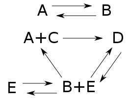
Here $A,B,C,D,$ and $E$ are names of chemicals, and the arrows are chemical reactions. If we know how fast each reaction goes, we can write down a 'rate equation' describing how the amount of each chemical changes with time.
In Part 17 we met the deficiency zero theorem, a powerful tool for finding equilibrium solutions of the rate equation: in other words, solutions where the amounts of the various chemicals don't change at all. To apply this theorem, two conditions must hold. Both are quite easy to check:
• Your reaction network needs to be 'weakly reversible': if you have a reaction that takes one bunch of chemicals to another, there's a series of reactions that takes that other bunch back to the one you started with.
• A number called the 'deficiency' that you can compute from your reaction network needs to be zero.
The first condition makes a lot of sense, intuitively: you won't get an equilibrium with all the different chemicals present if some chemicals can turn into others but not the other way around. But the second condition, and indeed the concept of 'deficiency', seems mysterious.
Luckily, when you work through the proof of the deficiency zero theorem, the mystery evaporates. It turns out that there are two equivalent ways to define the deficiency of a reaction network. One makes it easy to compute, and that's the definition people usually give. But the other explains why it's important.
In fact the whole proof of the deficiency zero theorem is full of great insights, so I want to show it to you. This will be the most intense part of the network theory series so far, but also the climax of its first phase. After a little wrapping up, we will then turn to another kind of network: electrical circuits!
Today I'll just unfold the concept of 'deficiency' so we see what it means. Next time I'll show you a slick way to write the rate equation, which is crucial to proving the deficiency zero theorem. Then we'll start the proof.
Let's recall what a reaction network is, and set up our notation. In chemistry we consider a finite set of 'species' like C, O2, H2O and so on... and then consider reactions like
On each side of this reaction we have a finite linear combination of species, with natural numbers as coefficients. Chemists call such a thing a complex.
So, given any finite collection of species, say $S$, let's write $\mathbb{N}^S$ to mean the set of finite linear combinations of elements of $S$, with natural numbers as coefficients. The complexes appearing in our reactions will form a subset of this, say $K$.
We'll also consider a finite collection of reactions---or in the language of Petri nets, 'transitions'. Let's call this $T$. Each transition goes from some complex to some other complex: if we want a reaction to be reversible we'll explicitly include another reaction going the other way. So, given a transition $\tau \in T$ it will always go from some complex called its source $s(\tau)$ to some complex called its target $t(\tau)$.
All this data, put together, is a reaction network:
Definition. A reaction network $(S,\; s,t : T \to K)$ consists of:
• a finite set $S$ of species,
• a finite set $T$ of transitions or reactions,
• a finite set $K \subset \mathbb{N}^S$ of complexes,
• source and target maps $s,t : T \to K$.
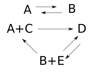
We can draw a reaction network as a graph with complexes as vertices and transitions as edges:
The set of species here is $S = \{A,B,C,D,E\}$, and the set of complexes is $K = \{A,B,D,A+C,B+E\}$.
But to write down the 'rate equation' describing our chemical reactions, we need a bit more information: constants $r(\tau)$ saying the rate at which each transition $\tau$ occurs. So, we define:
Definition. A stochastic reaction network is a reaction network $(S, \; s,t : T \to K)$ together with a map $r: T \to (0,\infty)$ assigning a rate constant to each transition.
Let me remind you how the rate equation works. At any time we have some amount $x_i \in [0,\infty)$ of each species $i$. These numbers are the components of a vector $x \in \mathbb{R}^S$, which of course depends on time. The rate equation says how this vector changes:
$$ \displaystyle{ \frac{d x_i}{d t} = \sum_{\tau \in T} r(\tau) \left(t_i(\tau) - s_i(\tau)\right) x^{s(\tau)} } $$
Here I'm writing $s_i(\tau)$ for the $i$th component of the vector $s(\tau)$, and similarly for $t_i(\tau)$. I should remind you what $x^{s(\tau)}$ means, since here we are raising a vector to a vector power, which is a bit unusual. So, suppose we have any vector $x = (x_1, \dots, x_k)$ and we raise it to the power of $s = (s_1, \dots, s_k)$. Then by definition we get
$$ \displaystyle{ x^s = x_1^{s_1} \cdots x_k^{s_k} } $$
Given this, I hope the rate equation makes intuitive sense! There's one term for each transition $\tau$. The factor of $t_i(\tau) - s_i(\tau)$ shows up because our transition destroys $s_i(\tau)$ things of the $i$th species and creates $t_i(\tau)$ of them. The big product
$$ \displaystyle{ x^{s(\tau)} = x_1^{s(\tau)_1} \cdots x_k^{s(\tau)_k} }$$
shows up because our transition occurs at a rate proportional to the product of the numbers of things it takes as inputs. The constant of proportionality is the reaction rate $r(\tau)$.
The deficiency zero theorem says lots of things, but in the next few episodes we'll prove a weak version, like this:
Deficiency Zero Theorem (Baby Version). Suppose we have a weakly reversible reaction network with deficiency zero. Then for any choice of rate constants there exists an equilibrium solution $x \in (0,\infty)^S$ of the rate equation. In other words:
$$ \displaystyle{ \sum_{\tau \in T} r(\tau) \left(t_i(\tau) - s_i(\tau)\right) x^{s(\tau)} = 0} $$
An important feature of this result is that all the components of the vector $x$ are positive. In other words, there's actually some chemical of each species present!
But what do the hypotheses in this theorem mean?
A reaction network is weakly reversible if for any transition $\tau \in T$ going from a complex $\kappa$ to a complex $\kappa'$, there is a sequence of transitions going from $\kappa'$ back to $\kappa$. But what about 'deficiency zero'? As I mentioned, this requires more work to understand.
So, let's dive in!
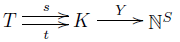
In modern math, we like to take all the stuff we're thinking about and compress it into a diagram with a few objects and maps going between these objects. So, to understand the deficiency zero theorem, I wanted to isolate the crucial maps. For starters, there's an obvious map
$$ Y : K \to \mathbb{N}^S $$
sending each complex to the linear combination of species that it is. We can think of $K$ as an abstract set equipped with this map saying how each complex is made of species, if we like. Then all the information in a stochastic reaction network sits in this diagram:
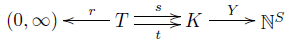
This is fundamental to everything we'll do for the next few episodes, so take a minute to lock it into your brain.
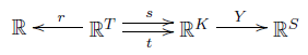
We'll do lots of different things with this diagram. For example, we often want to use ideas from linear algebra, and then we want our maps to be linear. For example, $Y$ extends uniquely to a linear map
$$ Y : \mathbb{R}^K \to \mathbb{R}^S $$
sending real linear combinations of complexes to real linear combinations of species. Reusing the name $Y$ here won't cause confusion. We can also extend $r$, $s$, and $t$ to linear maps in a unique way, getting a little diagram like this:
Linear algebra lets us talk about differences of complexes. Each transition $\tau$ gives a vector
$$ \partial \tau = t(\tau) - s(\tau)\in \mathbb{R}^K $$
saying the change in complexes that it causes. And we can extend $\partial$ uniquely to a linear map
$$ \partial : \mathbb{R}^T \to \mathbb{R}^K $$
defined on linear combinations of transitions. Mathematicians would call $\partial$ a boundary operator.
So, we have a little sequence of linear maps:
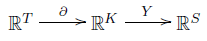
This turns a transition into a change in complexes, and then a change in species.
If you know fancy math you'll be wondering if this sequence is a 'chain complex', which is a fancy way of saying that $Y \partial = 0$. The answer is no. This equation means that every linear combination of reactions leaves the amount of all species unchanged. Or equivalently: every reaction leaves the amount of all species unchanged. This only happens in very silly examples.
Nonetheless, it's possible for a linear combination of reactions to leave the amount of all species unchanged.
For example, this will happen if we have a linear combination of reactions that leaves the amount of all complexes unchanged. But this sufficient condition is not necessary. And this leads us to the concept of 'deficiency zero':
Definition. A reaction network has deficiency zero if any linear combination of reactions that leaves the amount of every species unchanged also leaves the amount of every complex unchanged.
In short, a reaction network has deficiency zero iff
$$ Y (\partial \rho) = 0 \; \Rightarrow \; \partial \rho = 0 $$
for every $\rho \in \mathbb{R}^T$. In other words---using some basic concepts from linear algebra---a reaction network has deficiency zero iff $Y$ is one-to-one when restricted to the image of $\partial$. Remember, the image of $\partial$ is
$$ \mathrm{im} \partial = \{ \partial \rho \; : \; \rho \in \mathbb{R}^T \} $$
Roughly speaking, this consists of all changes in complexes that can occur due to reactions.
In still other words, a reaction network has deficiency zero if 0 is the only vector in both the image of $\partial$ and the kernel of $Y$:
$$ \mathrm{im} \partial \cap \mathrm{ker} Y = \{ 0 \} $$
Remember, the kernel of $Y$ is
$$ \mathrm{ker} Y = \{ \phi \in \mathbb{R}^K : Y \phi = 0 \} $$
Roughly speaking, this consists of all changes in complexes that don't cause changes in species. So, 'deficiency zero' roughly says that if a reaction causes a change in complexes, it causes a change in species.
(All this 'roughly speaking' stuff is because in reality I should be talking about linear combinations of transitions, complexes and species. But it's a bit distracting to keep saying that when I'm trying to get across the basic ideas!)
Now we're ready to understand deficiencies other than zero, at least a little. They're defined like this:
Definition. The deficiency of a reaction network is the dimension of $\mathrm{im} \partial \cap \mathrm{ker} Y$.
You can compute the deficiency of a reaction network just by looking at it. However, it takes a little training. First, remember that a reaction network can be drawn as a graph with complexes as vertices and transitions as edges, like this:
There are three important numbers we can extract from this graph:
• We can count the number of vertices in this graph; let's call that $|K|$, since it's just the number of complexes.
• We can count the number of pieces or 'components' of this graph; let's call that $\# \mathrm{components} $ for now.
• We can also count the dimension of the image of $Y \partial$. This space, $\mathrm{im} Y \partial$, is called the stoichiometric subspace: vectors in here are changes in species that can be accomplished by transitions in our reaction network, or linear combinations of transitions.
These three numbers, all rather easy to compute, let us calculate the deficiency:
Theorem. The deficiency of a reaction network equals
$$|K| - \# \mathrm{components} - \mathrm{dim} \left( \mathrm{im} Y \partial \right) $$
Proof. By definition we have
$$ \mathrm{deficiency} = \dim \left( \mathrm{im} \partial \cap \mathrm{ker} Y \right) $$
but another way to say this is
$$ \mathrm{deficiency} = \mathrm{dim} (\mathrm{ker} Y|_{\mathrm{im} \partial}) $$
where we are restricting $Y$ to the subspace $\mathrm{im} \partial$, and taking the dimension of the kernel of that.
The rank-nullity theorem says that whenever you have a linear map $T: V \to W$ between finite-dimensional vector spaces,
$$ \mathrm{dim} \left(\mathrm{ker} T \right) \; = \; \mathrm{dim}\left(\mathrm{dom} T\right) \; - \; \mathrm{dim} \left(\mathrm{im} T\right) $$
where $\mathrm{dom} T$ is the domain of $T$, namely the vector space $V$. It follows that
$$ \mathrm{dim}(\mathrm{ker} Y|_{\mathrm{im} \partial}) = \mathrm{dim}(\mathrm{dom} Y|_{\mathrm{im} \partial}) - \mathrm{dim}(\mathrm{im} Y|_{\mathrm{im} \partial}) $$
The domain of $Y|_{\mathrm{im} \partial}$ is just $\mathrm{im} \partial$, while its image equals $\mathrm{im} Y \partial$, so
$$ \mathrm{deficiency} = \mathrm{dim}(\mathrm{im} \partial) - \mathrm{dim}(\mathrm{im} Y \partial) $$
The theorem then follows from this:
Lemma. $ \mathrm{dim} (\mathrm{im} \partial) = |K| - \# \mathrm{components} $.
Proof. In fact this holds whenever we have a finite set of complexes and a finite set of transitions going between them. We get a diagram

We can extend the source and target functions to linear maps as usual:
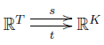
and then we can define $\partial = t - s$. We claim that
$$ \mathrm{dim} (\mathrm{im} \partial) = |K| - \# \mathrm{components} $$
where $\# \mathrm{components}$ is the number of connected components of the graph with $K$ as vertices and $T$ as edges.
This is easiest to see using an inductive argument where we start by throwing out all the edges of our graph and then put them back in one at a time. When our graph has no edges, $\partial = 0$ and the number of components is $|K|$, so our claim holds: both sides of the equation above are zero. Then, each time we put in an edge, there are two choices: either it goes between two different components of the graph we have built so far, or it doesn't. If goes between two different components, it increases $\mathrm{dim} (\mathrm{im} \partial$ by 1 and decreases the number of components by 1, so our equation continues to hold. If it doesn't, neither of these quantities change, so our equation again continues to hold. █
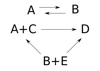
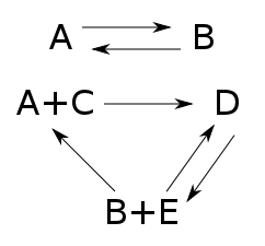
This reaction network is not weakly reversible, since we can get from $B + E$ and $A + C$ to $D$ but not back. It becomes weakly reversible if we throw in another transition:
Taking a reaction network and throwing in the reverse of an existing transition never changes the number of complexes, the number of components, or the dimension of the stoichiometric subspace. So, the deficiency of the reaction network remains unchanged. We computed it back in Part 17. For either reaction network above:
• the number of complexes is 5:
$$ |K| = |\{A,B,D, A+C, B+E\}| = 5 $$
• the number of components is 2:
$$ \# \mathrm{components} = 2 $$
• the dimension of the stoichometric subspace is 3. For this we go through each transition, see what change in species it causes, and take the vector space spanned by these changes. Then we find a basis for this space and count it:
$$ \begin{array}{ccl} \mathrm{im} Y\partial &=& \langle B-A, A-B, D - A - C, D - (B+E) , (B+E)-(A+C) \rangle \\ &=& \langle B -A, D - A - C, D - A - E \rangle \end{array} $$
so
$$ \mathrm{dim} \left(\mathrm{im} Y\partial \right) = 3 $$
As a result, the deficiency is zero:
$$ \begin{array}{ccl} \mathrm{deficiency} &=& |K| - \# \mathrm{components} - \mathrm{dim} \left( \mathrm{im} Y\partial \right) \\ &=& 5 - 2 - 3 \\ &=& 0 \end{array} $$
Now let's throw in another complex and some more transitions:
Now:
• the number of complexes increases by 1:
$$ |K| = |\{A,B,D,E, A+C, B+E\}| = 6 $$
• the number of components is unchanged:
$$ \# \mathrm{components} = 2 $$
• the dimension of the stoichometric subspace increases by 1. We never need to include reverses of transitions when computing this:
$$ \begin{array}{ccl} \mathrm{im} Y\partial &=& \langle B-A, E-B, D - (A+C), D - (B+E) , (B+E)-(A+C) \rangle \\ &=& \langle B -A, E-B, D - A - C, D - B - E \rangle \end{array} $$
so
$$ \mathrm{dim} \left(\mathrm{im} Y\partial \right) = 4 $$
As a result, the deficiency is still zero:
$$ \begin{array}{ccl} \mathrm{deficiency} &=& |K| - \# \mathrm{components} - \mathrm{dim} \left( \mathrm{im} Y\partial \right) \\ &=& 6 - 2 - 4 \\ &=& 0 \end{array} $$
Do all reaction networks have deficiency zero? That would be nice. Let's try one more example:
• the number of complexes is the same as in our last example:
$$ |K| = |\{A,B,D,E, A+C, B+E\}| = 6 $$
• the number of components is also the same:
$$ \# \mathrm{components} = 2 $$
• the dimension of the stoichometric subspace is also the same:
$$ \begin{array}{ccl} \mathrm{im} Y\partial &=& \langle B-A, D - (A+C), D - (B+E) , (B+E)-(A+C), (B+E) - B \rangle \\ &=& \langle B -A, D - A - C, D - B , E\rangle \end{array} $$
so
$$ \mathrm{dim} \left(\mathrm{im} Y\partial \right) = 4 $$
So the deficiency is still zero:
$$ \begin{array}{ccl} \mathrm{deficiency} &=& |K| - \# \mathrm{components} - \mathrm{dim} \left( \mathrm{im} Y\partial \right) \\ &=& 6 - 2 - 4 \\ &=& 0 \end{array} $$
It's sure easy to find examples with deficiency zero!
Puzzle 1. Can you find an example where the deficiency is not zero?
Puzzle 2. If you can't find an example, prove the deficiency is always zero. If you can, find 1) the smallest example and 2) the smallest example that actually arises in chemistry.
Note that not all reaction networks can actually arise in chemistry. For example, the transition $A \to A + A$ would violate conservation of mass. Nonetheless a reaction network like this might be useful in a very simple model of amoeba reproduction, one that doesn't take limited resources into account.
I'll conclude with some technical remarks that only a mathematician could love; feel free to skip them if you're not in the mood. As you've already seen, it's important that a reaction network can be drawn as a graph:
But there are many kinds of graph. What kind of graph is this, exactly?
As I mentioned in Part 17, it's a directed multigraph, meaning that the edges have arrows on them, more than one edge can go from one vertex to another, and we can have any number of edges going from a vertex to itself. Not all those features are present in this example, but they're certainly allowed by our definition of reaction network!
After all, we've seen that a stochastic reaction network amounts to a little diagram like this:
If we throw out the rate constants, we're left with a reaction network. So, a reaction network is just a diagram like this:
If we throw out the information about how complexes are made of species, we're left with an even smaller diagram:
And this precisely matches the slick definition of a directed multigraph: it's a set $E$ of edges, a set $V$ of vertices, and functions $s,t : E \to V$ saying where each edge starts and where it ends: its source and target.
Since this series is about networks, we should expect to run into many kinds of graphs. While their diversity is a bit annoying at first, we must learn to love it, at least if we're mathematicians and want everything to be completely precise.
There are at least 23 = 8 kinds of graphs, depending on our answers to three questions:
• Do the edges have arrows on them?
• Can more than one edge can go between a specific pair of vertices?
and
• Can an edge can go from a vertex to itself?
We get directed multigraphs if we answer YES, YES and YES to these questions. Since they allow all three features, directed multigraphs are very important. For example, a category is a directed multigraph equipped with some extra structure. Also, what mathematicians call a quiver is just another name for a directed multigraph.
We've met two other kinds of graph so far:
• In Part 15 and Part 16 we described circuits made of resistors—or, in other words, Dirichlet operators—using 'simple graphs'. We get simple graphs when we answer NO, NO and NO to the three questions above. The slick definition of a simple graph is that it's a set $V$ of vertices together with a subset $E$ of the collection of 2-element subsets of $V$.
• In Part 20 we described Markov processes on finite sets—or, in other words, infinitesimal stochastic operators—using 'directed graphs'. We get directed graphs when we answer YES, NO and YES to the three questions. The slick definition of a directed graph is that it's a set $V$ of vertices together with a subset $E$ of the ordered pairs of $V$:
$$ E \subseteq V \times V$$
There is a lot to say about this business, but for now I'll just note that you can use directed multigraphs with edges labelled by positive numbers to describe Markov processes, just as we used directed graphs. You don't get anything more general, though! After all, if we have multiple edges from one vertex to another, we can replace them by a single edge as long as we add up their rate constants. And an edge from a vertex to itself has no effect at all.
In short, both for Markov processes and reaction networks, we can take 'graph' to mean either 'directed graph' or 'directed multigraph', as long as we make some minor adjustments. In what follows, we'll use directed multigraphs for both Markov processes and reaction networks. It will work a bit better if we ever get around to explaining how category theory fits into this story.
You can also read comments on Azimuth, and make your own comments or ask questions there!
|
|
|
|