

|
|
|
|
But first, let me quickly sketch why it could be worthwhile.
Consider this stochastic Petri net with rate constant $r$:
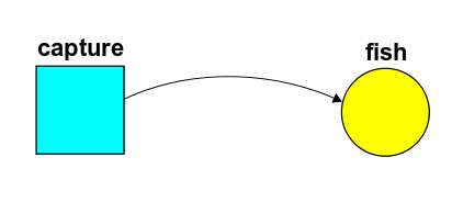
Problem. Suppose we start out knowing for sure there are no fish in the fisherman's net. What's the probability that he has caught $n$ fish at time $t$?
At any time there will be some probability of having caught $n$ fish; let's call this probability $\psi(n,t)$. We can summarize all these probabilities in a single power series, called a generating function: $$\Psi(t) = \sum_{n=0}^\infty \psi(n,t) \, z^n $$
Here $latex z$ is a formal variable—don't ask what it means, for now it's just a trick. In quantum theory we use this trick when talking about collections of photons rather than fish, but then the numbers $\psi(n,t)$ are complex 'amplitudes'. Now they are real probabilities, but we can still copy what the physicists do, and use this trick to rewrite the master equation as follows:
$$\frac{d}{d t} \Psi(t) = H \Psi(t) $$
This describes how the probability of having caught any given number of fish changes with time.
What's the operator $H$? Well, in quantum theory we describe the creation of photons using a certain operator on power series called the creation operator:
$$a^\dagger \Psi = z \Psi $$
We can try to apply this to our fish. If at some time we're 100% sure we have $n$ fish, we have
$$\Psi = z^n$$
so applying the creation operator gives
$$a^\dagger \Psi = z^{n+1}$$
One more fish! That's good. So, an obvious wild guess is
$$H = r a^\dagger$$
where $r$ is the rate at which we're catching fish. Let's see how well this guess works.
If you know how to exponentiate operators, you know to solve this equation:
$$\frac{d}{d t} \Psi(t) = H \Psi(t) $$
It's easy:
$$\Psi(t) = \mathrm{exp}(t H) \Psi(0)$$
Since we start out knowing there are no fish in the net, we have
$$\Psi(0) = 1$$
so with our guess for $H$ we get
$$\Psi(t) = \mathrm{exp}(r t a^\dagger) 1$$
But $a^\dagger$ is the operator of multiplication by $z$, so $\mathrm{exp}(r t a^\dagger)$ is multiplication by $e^{r t z}$, and
$$\Psi(t) = e^{r t z} = \sum_{n = 0}^\infty \frac{(r t)^n}{n!} \, z^n$$
So, if our guess is right, the probability of having caught $n$ fish at time $t$ is
$$\frac{(r t)^n}{n!}$$
Unfortunately, this can't be right, because these probabilities don't sum to 1! Instead their sum is
$$\sum_{n=0}^\infty \frac{(r t)^n}{n!} = e^{r t}$$
We can try to wriggle out of the mess we're in by dividing our answer by this fudge factor. It sounds like a desperate measure, but we've got to try something!
This amounts to guessing that the probability of having caught $n$ fish by time $t$ is
$$\frac{(r t)^n}{n!} \, e^{-r t }$$
And this is right! This is called the Poisson distribution: it's famous for being precisely the answer to the problem we're facing.
So on the one hand our wild guess about $H$ was wrong, but on the other hand it was not so far off. We can fix it as follows:
$$H = r (a^\dagger - 1)$$
The extra $-1$ gives us the fudge factor we need.
So, a wild guess corrected by an ad hoc procedure seems to have worked! But what's really going on?
What's really going on is that $a^\dagger$, or any multiple of this, is not a legitimate Hamiltonian for a master equation: if we define a time evolution operator $\exp(t H)$ using a Hamiltonian like this, probabilities won't sum to 1! But $a^\dagger - 1$ is okay. So, we need to think about which Hamiltonians are okay.
In quantum theory, self-adjoint Hamiltonians are okay. But in probability theory, we need some other kind of Hamiltonian. Let's figure it out.
• In a probabilistic model, we may instead say that the system has a probability $\psi(x)$ of being in any state $x \in X$. These probabilities are nonnegative real numbers with
$$\sum_{x \in X} \psi(x) = 1$$
• In a quantum model, we may instead say that the system has an amplitude $\psi(x)$ of being in any state $x \in X$. These amplitudes are complex numbers with
$$\sum_{x \in X} | \psi(x) |^2 = 1$$
Probabilities and amplitudes are similar yet strangely different. Of course given an amplitude we can get a probability by taking its absolute value and squaring it. This is a vital bridge from quantum theory to probability theory. Today, however, I don't want to focus on the bridges, but rather the parallels between these theories.
We often want to replace the sums above by integrals. For that we need to replace our set $X$ by a measure space, which is a set equipped with enough structure that you can integrate real or complex functions defined on it. Well, at least you can integrate so-called 'integrable' functions—but I'll neglect all issues of analytical rigor here. Then:
• In a probabilistic model, the system has a probability distribution $\psi : X \to \mathbb{R}$, which obeys $\psi \ge 0$ and
$$\int_X \psi(x) \, d x = 1$$
• In a quantum model, the system has a wavefunction $\psi : X \to \mathbb{C}$, which obeys
$$\int_X | \psi(x) |^2 \, d x= 1$$
In probability theory, we integrate $\psi$ over a set $S \subset X$ to find out the probability that our systems state is in this set. In quantum theory we integrate $|\psi|^2$ over the set to answer the same question.
We don't need to think about sums over sets and integrals over measure spaces separately: there's a way to make any set $X$ into a measure space such that by definition,
$$\int_X \psi(x) \, dx = \sum_{x \in X} \psi(x)$$
In short, integrals are more general than sums! So, I'll mainly talk about integrals, until the very end.
In probability theory, we want our probability distributions to be vectors in some vector space. Ditto for wave functions in quantum theory! So, we make up some vector spaces:
• In probability theory, the probability distribution $\psi$ is a vector in the space
$$L^1(X) = \{ \psi: X \to \mathbb{C} \; : \; \int_X |\psi(x)| \, d x < \infty \} $$
• In quantum theory, the wavefunction $\psi$ is a vector in the space
$$L^2(X) = \{ \psi: X \to \mathbb{C} \; : \; \int_X |\psi(x)|^2 \, d x < \infty \} $$
You may wonder why I defined $L^1(X)$ to consist of complex functions when probability distributions are real. I'm just struggling to make the analogy seem as strong as possible. In fact probability distributions are not just real but nonnegative. We need to say this somewhere... but we can, if we like, start by saying they're complex-valued functions, but then whisper that they must in fact be nonnegative (and thus real). It's not the most elegant solution, but that's what I'll do for now.
Now:
• The main thing we can do with elements of $L^1(X)$, besides what we can do with vectors in any vector space, is integrate one. This gives a linear map:
$$\int : L^1(X) \to \mathbb{C} $$
• The main thing we can with elements of $L^2(X)$, besides the besides the things we can do with vectors in any vector space, is take the inner product of two:
$$\langle \psi, \phi \rangle = \int_X \overline{\psi}(x) \phi(x) \, d x $$
This gives a map that's linear in one slot and conjugate-linear in the other:
$$\langle - , - \rangle : L^2(X) \times L^2(X) \to \mathbb{C} $$
First came probability theory with $L^1(X)$; then came quantum theory with $L^2(X)$. Naive extrapolation would say it's about time for someone to invent an even more bizarre theory of reality based on $L^3(X).$ In this, you'd have to integrate the product of three wavefunctions to get a number! The math of Lp spaces is already well-developed, so give it a try if you want. I'll stick to $L^1$ and $L^2$ today.
Now let's think about time evolution:
• In probability theory, the passage of time is described by a map sending probability distributions to probability distributions. This is described using a stochastic operator
$$U : L^1(X) \to L^1(X)$$
meaning a linear operator such that
$$\int U \psi = \int \psi $$
and
$$\psi \ge 0 \quad \Rightarrow \quad U \psi \ge 0$$
• In quantum theory the passage of time is described by a map sending wavefunction to wavefunctions. This is described using an isometry
$$U : L^2(X) \to L^2(X)$$
meaning a linear operator such that
$$\langle U \psi , U \phi \rangle = \langle \psi , \phi \rangle $$
In quantum theory we usually want time evolution to be reversible, so we focus on isometries that have inverses: these are called unitary operators. In probability theory we often consider stochastic operators that are not invertible.
Sometimes it's nice to think of time coming in discrete steps. But in theories where we treat time as continuous, to describe time evolution we usually need to solve a differential equation. This is true in both probability theory and quantum theory:
• In probability theory we often describe time evolution using a differential equation called the master equation:
$$\frac{d}{d t} \psi(t) = H \psi(t) $$
whose solution is
$$\psi(t) = \exp(t H)\psi(0) $$
• In quantum theory we often describe time evolution using a differential equation called Schrödinger's equation:
$$i \frac{d}{d t} \psi(t) = H \psi(t) $$
whose solution is
$$\psi(t) = \exp(-i t H)\psi(0) $$
In fact the appearance of $i$ in the quantum case is purely conventional; we could drop it to make the analogy better, but then we'd have to work with 'skew-adjoint' operators instead of self-adjoint ones in what follows.
Let's guess what properties an operator $H$ should have to make $\exp(-i t H)$ unitary for all $t$. We start by assuming it's an isometry:
$$\langle \exp(-i t H) \psi, \exp(-i t H) \phi \rangle = \langle \psi, \phi \rangle$$
Then we differentiate this with respect to $t$ and set $t = 0$, getting
$$\langle -i H \psi, \phi \rangle + \langle \psi, -i H \phi \rangle = 0$$
or in other words:
$$\langle H \psi, \phi \rangle = \langle \psi, H \phi \rangle $$
Physicists call an operator obeying this condition self-adjoint. Mathematicians know there's more to it, but today is not the day to discuss such subtleties, intriguing though they be. All that matters now is that there is, indeed, a correspondence between self-adjoint operators and well-behaved 'one-parameter unitary groups' $\exp(-i t H)$. This is called Stone's Theorem.
But now let's copy this argument to guess what properties an operator $H$ must have to make $\exp(t H)$ stochastic. We start by assuming $\exp(t H)$ is stochastic, so
$$\int \exp(t H) \psi = \int \psi $$
and
$$\psi \ge 0 \quad \Rightarrow \quad \exp(t H) \psi \ge 0$$
We can differentiate the first equation with respect to $t$ and set $t = 0$, getting
$$\int H \psi = 0$$
for all $\psi$.
But what about the second condition,
$$\psi \ge 0 \quad \Rightarrow \quad \exp(t H) \psi \ge 0? $$
It seems easier to deal with this in the special case when integrals over $X$ reduce to sums. So let's suppose that happens... and let's start by seeing what the first condition says in this case.
In this case, $L^1(X)$ has a basis of 'Kronecker delta functions': The Kronecker delta function $\delta_i$ vanishes everywhere except at one point $i \in X$, where it equals 1. Using this basis, we can write any operator on $L^1(X)$ as a matrix.
As a warmup, let's see what it means for an operator
$$U: L^1(X) \to L^1(X)$$
to be stochastic in this case. We'll take the conditions
$$\int U \psi = \int \psi $$
and
$$\psi \ge 0 \quad \Rightarrow \quad U \psi \ge 0$$
and rewrite them using matrices. For both, it's enough to consider the case where $\psi$is a Kronecker delta, say $\delta_j$.
In these terms, the first condition says
$$\sum_{i \in X} U_{i j} = 1 $$
for each column $j$. The second says
$$ U_{i j} \ge 0$$
for all $i, j$. So in this case, a stochastic operator is just a square matrix where each column sums to 1 and all the entries are nonnegative. (Such matrices are often called left stochastic.)
Next, let's see what we need for an operator $H$ to have the property that $\exp(t H)$is stochastic for all $t \ge 0$. It's enough to assume $t$ is very small, which lets us use the approximation
$$\exp(t H) = 1 + t H + \cdots $$
and work to first order in $t$. Saying that each column of this matrix sums to 1 then amounts to
$$\sum_{i \in X} \delta_{i j} + t H_{i j} + \cdots = 1$$
which requires
$$ \sum_{i \in X} H_{i j} = 0$$
Saying that each entry is nonnegative amounts to
$$\delta_{i j} + t H_{i j} + \cdots \ge 0$$
When $i = j$ this will be automatic when $t$ is small enough, so the meat of this condition is
$$H_{i j} \ge 0 \; \mathrm{if} \; i \ne j$$
So, let's say $H$ is an infinitesimal stochastic matrix if its columns sum to zero and its off-diagonal entries are nonnegative.
I don't love this terminology: do you know a better one? There should be some standard term. People here say they've seen such an operator called a 'stochastic Hamiltonian'. The idea behind my term is that any infinitesimal stochastic operator should be the infinitesimal generator of a stochastic process.
In other words, when we get the details straightened out, any 1-parameter family of stochastic operators $$ U(t) : L^1(X) \to L^1(X) \qquad t \ge 0 $$ obeying $$ U(0) = I $$ $$ U(t) U(s) = U(t+s) $$ and continuity: $$ t_i \to t \quad \Rightarrow \quad U(t_i) \psi \to U(t)\psi $$ should be of the form $$ U(t) = \exp(t H)$$ for a unique 'infinitesimal stochastic operator' $H$.
When $X$ is a finite set, this is true—and an infinitesimal stochastic operator is just a square matrix whose columns sum to zero and whose off-diagonal entries are nonnegative. But do you know a theorem characterizing infinitesimal stochastic operators for general measure spaces $X$? Someone must have worked it out.
Luckily, for our work on stochastic Petri nets, we only need to understand the case where $X$ is a countable set and our integrals are really just sums. This should be almost like the case where $X$ is a finite set—but we'll need to take care that all our sums converge.
In this example, our set of states is the natural numbers:
$$X = \mathbb{N}$$
The probability distribution
$$\psi : \mathbb{N} \to \mathbb{C}$$
tells us the probability of having caught any specific number of fish.
The creation operator is not infinitesimal stochastic: in fact, it's stochastic! Why? Well, when we apply the creation operator, what was the probability of having $n$ fish now becomes the probability of having $n+1$ fish. So, the probabilities remain nonnegative, and their sum over all $n$ is unchanged. Those two conditions are all we need for a stochastic operator.
Using our fancy abstract notation, these conditions say:
$$\int a^\dagger \psi = \int \psi $$
and
$$ \psi \ge 0 \; \Rightarrow \; a^\dagger \psi \ge 0 $$
So, precisely by virtue of being stochastic, the creation operator fails to be infinitesimal stochastic:
$$ \int a^\dagger \psi \ne 0 $$
Thus it's a bad Hamiltonian for our stochastic Petri net.
On the other hand, $a^\dagger - 1$ is infinitesimal stochastic. Its off-diagonal entries are the same as those of $a^\dagger$, so they're nonnegative. Moreover:
$$ \int (a^\dagger - 1) \psi = 0 $$
precisely because
$$\int a^\dagger \psi = \int \psi $$
You may be thinking: all this fancy math just to understand a single stochastic Petri net, the simplest one of all!
But next time I'll explain a general recipe which will let you write down the Hamiltonian for any stochastic Petri net. The lessons we've learned today will make this much easier. And pondering the analogy between probability theory and quantum theory will also be good for our bigger project of unifying the applications of network diagrams to dozens of different subjects.
You can also read comments on Azimuth, and make your own comments or ask questions there!
|
|
|
|