


|
|
|
|
It's not a realistic model; we're just getting started. But some programmers in the Azimuth Project team are interested in making more such models—especially Allan Erskine (who made this one), Jim Stuttard (who helped me get it to work), Glyn Adgie and Staffan Liljgeren. It could be a fun way for us to learn and explain climate physics. With enough of these models, we'd have a whole online course! If you want to help us out, please say hi.
Allan will say more about the programming challenges later. But first, a big puzzle: how can small changes in the Earth's orbit lead to big changes in the Earth's climate? As I mentioned last time, it seems hard to understand the glacial cycles of the last few million years without answering this.
Are there feedback mechanisms that can amplify small changes in temperature? Yes. Here are a few obvious ones:
Ice albedo feedback. Snow and ice reflect more light than liquid oceans or soil. When the Earth warms up, snow and ice melt, so the Earth becomes darker, absorbs more light, and tends to get get even warmer. Conversely, when the Earth cools down, more snow and ice form, so the Earth becomes lighter, absorbs less light, and tends to get even cooler.
See week302 for more on feedbacks and how big they're likely to be.
On top of all these subtleties, any proposed solution to the puzzle of glacial cycles needs to keep a few other things in mind, too:
The classic example of a bistable system is a switch—say for an electric light. When the light is on it stays on; when the light is off it stays off. If you touch the switch very gently, nothing will happen. But if you push on it hard enough, it will suddenly pop from on to off, or vice versa.
If we're trying to model the glacial cycles using this idea, we need the switch to have a fairly dramatic effect, yet still be responsive to a fairly gentle touch. For this to work we need enough positive feedback... but not too much.
(We could also try a different idea: maybe the Earth keeps itself in its icy glacial state, or its warm interglacial state, using some mechanism that gradually uses something up. Then, when the Earth runs out of this stuff, whatever it is, the climate can easily flip to the other state.)
For these and other reasons, any solution to the ice age puzzle is bound to be subtle. Instead of diving straight into this complicated morass, let's try something much simpler. Let's just think about how the ice albedo effect could, in theory, make the Earth bistable.
To do this, let's look at the very simplest model in this great not-yet-published book:
This is a zero-dimensional energy balance model, meaning that it only involves the average temperature of the earth, the average solar radiation coming in, and the average infrared radiation going out.
The average temperature will be \(T\), measured in Celsius. We'll assume the Earth radiates power square meter equal to $$ \displaystyle{ A + B T }$$ where \(A\) = 218 watts/meter2 and \(B\) = 1.90 watts/meter2 per degree Celsius. This is a linear approximation taken from satellite data on our Earth. In reality, the power emitted grows faster than linearly with temperature.
We'll assume the Earth absorbs solar energy power per square meter equal to
$$ Q c(T) $$Here:
Why a quarter? That's a nice geometry puzzle: we worked it out at the Azimuth Blog once.
\(c(T)\) is the coalbedo: the fraction of solar power that gets absorbed. The coalbedo depends on the temperature; we'll have to say how.
Given all this, we get
$$ C \frac{d T}{d t} = - A - B T + Q c(T(t)) $$where \(C\) is Earth's heat capacity in joules per degree per square meter. Of course this is a funny thing, because heat energy is stored not only at the surface but also in the air and/or water, and the details vary a lot depending on where we are. But if we consider a uniform planet with dry air and no ocean, North says we may roughly take \(C\) equal to about half the heat capacity at constant pressure of the column of dry air over a square meter, namely 5 million joules per degree Celsius.
The easiest thing to do is find equilibrium solutions, meaning solutions where \(\frac{d T}{d t} = 0\), so that
$$ A + B T = Q c(T) $$Now \(C\) doesn't matter anymore! We'd like to solve for \(T\) as a function of the insolation \(Q\), but it's easier to solve for \(Q\) as a function of \(T\): $$ Q = \frac{ A + B T } {c(T) }$$ To go further, we need to guess some formula for the coalbedo \(c(T)\). The coalbedo, remember, is the fraction of sunlight that gets absorbed when it hits the Earth. It's 1 minus the albedo, which is the fraction that gets reflected. Here's a little chart of albedos:

If you get mixed up between albedo and coalbedo, just remember: coal has a high coalbedo.
Since we're trying to keep things very simple right not, not model nature in all its glorious complexity, let's just say the average albedo of the Earth is 0.65 when it's very cold and there's lots of snow. So, let
$$ c_i = 1 - 0.65 = 0.35 $$be the 'icy' coalbedo, good for very low temperatures. Similarly, let's say the average albedo drops to 0.3 when its very hot and the Earth is darker. So, let $$ c_f = 1 - 0.3 = 0.7 $$
be the 'ice-free' coalbedo, good for high temperatures when the Earth is darker.
Then, we need a function of temperature that interpolates between \(c_i\) and \(c_f\). Let's try this:
$$ c(T) = c_i + \frac{1}{2} (c_f-c_i) (1 + \tanh(\gamma T)) $$If you're not a fan of the hyperbolic tangent function \(\tanh\), this may seem scary. But don't be intimidated!
The function \(\frac{1}{2}(1 + \tanh(\gamma T)) \) is just a function that goes smoothly from 0 at low temperatures to 1 at high temperatures. This ensures that the coalbedo is near its icy value \(c_i\) at low temperatures, and near its ice-free value \(c_f\) at high temperatures. But the fun part here is \(\gamma\), a parameter that says how rapidly the coalbedo rises as the Earth gets warmer. Depending on this, we'll get different effects!
The function \(c(T)\) rises fastest at \(T = 0\), since that's where \(\tanh (\gamma T)\) has the biggest slope. We're just lucky that in Celsius \(T = 0\) is the melting point of ice, so this makes a bit of sense.
Now Allan Erskine's programming magic comes into play! You can slide this slider to adjust the parameter \(\gamma\) to various values between 0 and 1:
You can see how the coalbedo \(c(T)\) changes as a function of the temperature \(T\). In this graph the temperature ranges from -50 °C and 50 °C; the graph depends on what value of \(\gamma\) you choose with the slider:
Here's the insolation \(Q\) required to yield a given temperature \(T\) between -50 °C and 50 °C:
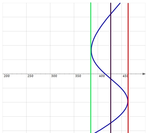
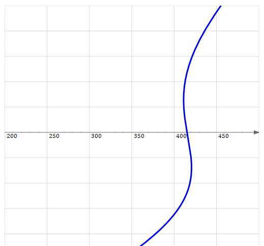
It's easiest to solve for \(Q\) in terms of \(T\). But it's more intuitive to flip this graph over and see what equilibrium temperatures \(T\) are allowed for a given insolation \(Q\) between 200 and 500 watts per square mater:
The exciting thing is that when \(\gamma\) gets big enough, three different temperatures are compatible with the same amount of insolation! This means the Earth can be hot, cold or something intermediate even when the amount of sunlight hitting it is fixed. The intermediate state is unstable, it turns out. Only the hot and cold states are stable. So, we say the Earth is bistable in this simplified model.
Can you see how big \(\gamma\) needs to be for this bistability to kick in? It's certainly there when \(\gamma = 0.05\), since then we get a graph like this:
Why is the intermediate state unstable when it exists? Why are the other two equilibria stable? To answer these questions, we'd need to go back and study the original equation:
$$ C \frac{d T}{d t} = - A - B T + Q c(T(t)) $$and see what happens when we push \(T\) slightly away from one of its equilibrium values. That's really fun, but we won't do it today. Instead, let's draw some conclusions from what we've just seen. There are at least three morals: a mathematical moral, a climate science model, and a software moral.
Mathematically, this model illustrates catastrophe theory. As we slowly turn up \(\gamma\), we get different curves showing how temperature is a function of insolation... until suddenly the curve isn't the graph of a function anymore: it becomes infinitely steep at one point! After that, we get bistability:
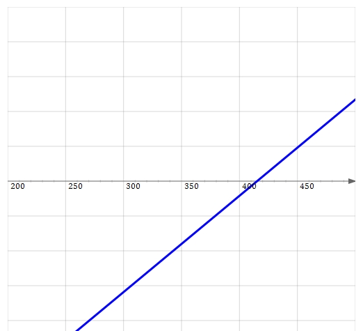
\(\gamma = 0.01 \)
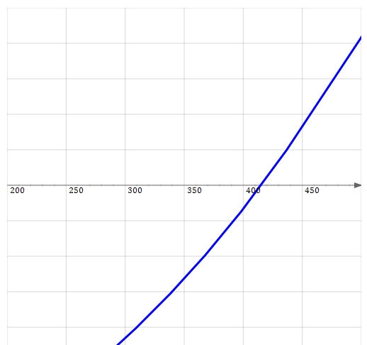
\(\gamma = 0.02 \)
\(\gamma = 0.03 \)
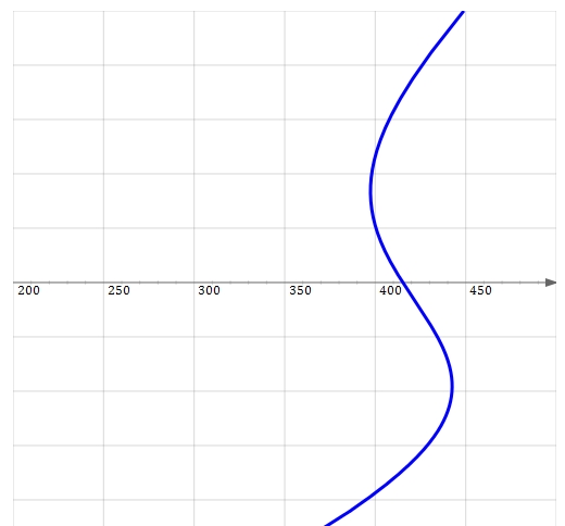
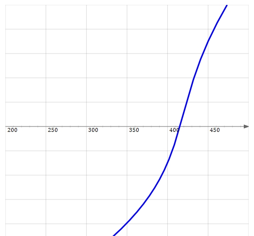
\(\gamma = 0.04 \)
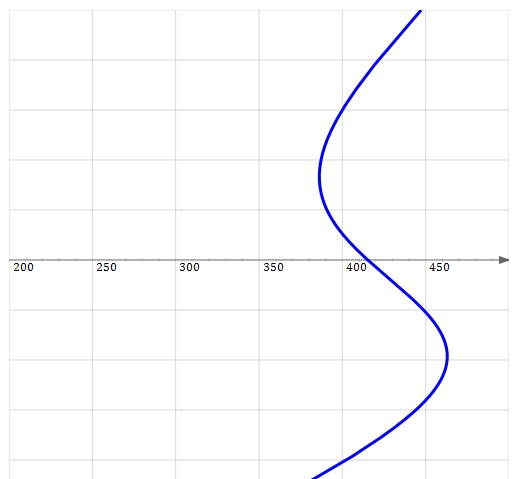
\(\gamma = 0.05 \)
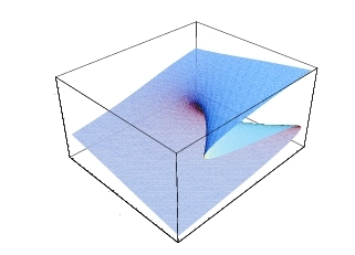
This is called a cusp catastrophe, and you can visualize these curves as slices of a surface in 3d, which looks roughly like this picture:
As far as climate science goes, one moral is that it pays to spend some time making sure we understand simple models before we dive into more complicated ones. Right now we're looking at a very simple model, but we're already seeing some interesting phenomena. The kind of model we're looking at now is called a Budyko-Sellers model. These have been studied since the late 1960's:
It also pays to compare our models to reality! For example, the graphs we've seen show some remarkably hot and cold temperatures for the Earth. That's a bit unnerving. Let's investigate. Suppose we set \(\gamma = 0\) on our slider. Then the coalbedo of the Earth becomes independent of temperature: it's 0.525, halfway between its icy and ice-free values. Then, when the insolation takes its actual value of 342.5 watts per square meter, the model says the Earth's temperature is very chilly: about -20 °C!
Does that mean the model is fundamentally flawed? Maybe not! After all, it's based on very light-colored Earth. Suppose we use the actual albedo of the Earth. Of course that's hard to define, much less determine. But let's just look up some average value of the Earth's albedo: supposedly it's about 0.3. That gives a coalbedo of \(c = 0.7\). If we plug that in our formula:
$$ Q = \frac{ A + B T } {c}$$we get 11 °C. That's not too far from the Earth's actual average temperature, namely about 15 ° C. So the chilly temperature of -20 °C seems to come from an Earth that's a lot lighter in color than ours.
Our model includes the greenhouse effect, since the coeficients \(A\) and \(B\) were determined by satellite measurements of how much radiation actually escapes the Earth's atmosphere and shoots out into space. As a further check to our model, we can look at an even simpler zero-dimensional energy balance model: a completely black Earth with no greenhouse effect. Another member of the Azimuth Project has written about this:
As he explains, this model gives the Earth a temperature of 6 °C. He also shows that in this model, lowering the albedo to a realistic value of 0.3 lowers the temperature to a chilly -18 ° C. To get from that to something like our Earth, we must take the greenhouse effect into account.
This sort of fiddling around is the sort of thing we must do to study the flaws and virtues of a climate model. Of course, any realistic climate model is vastly more sophisticated than the little toy we've been looking at, so the 'fiddling around' must also be more sophisticated. With a more sophisticated model, we can also be more demanding. For example, when I said 11 °C is "is not too far from the Earth's actual average temperature, namely about 15 ° C", I was being very blasé about what's actually a big discrepancy. I only took that attitude because the calculations we're doing now are very preliminary.
Finally, here's what Allan has to say about the software you've just seen, and some fancier software you'll see in forthcoming weeks:
Your original question in the Azimuth Forum was "What's the easiest way to write simple programs of this sort that could be accessed and operated by clueless people online?" A "simple program" for the climate model you proposed needed two elements: a means to solve the ODE (ordinary differential equation) describing the model, and a means to interact with and visualize the results for the (clearly) "clueless people online".
Some good suggestions were made by members of the forum:
- use a full-fledged numerical computing package such as Sage or Matlab which come loaded to the teeth with ODE solvers and interactive charting;
- use a full-featured programming language like Java which has libraries available for ode solving and charting, and which can be packaged as an applet for the web;
- do all the computation and visualization ourselves in Javascript.
While the first two suggestions were superior for computing the ODE solutions, I knew from bitter experience (as a software developer) that the truly clueless people were us bold forum members engaged in this new online enterprise: none of us were experts in this interactive/online math thing, and programming new software is almost always harder than you expect it to be.
Then actually releasing new software is harder still! Especially to an audience as large as your readership. To come up an interactive solution that would work on many different computers/browsers, the most mundane and pedestrian suggestion of "do it all ourselves in Javascript and have them run it in the browser" was also the most likely to be a success.
The issue with Javascript was that not many people use it for numerical computation, and I was down on our chances of success until Staffan pointed out the excellent JSXGraph software. JSXGraph has many examples available to get up and running, has an ODE solver, and after a copy/paste or two and some tweaking on my part we were all set.
The true vindication for going all-Javascript though was that you were subsequently able to do some copy/pasting of your own directly into TWF without any servers needing configured etc., or even any help from me! The graphs ought to be viewable by your readership for as long as browsers support Javascript (a sign of a good software release is that you don't have to think about it afterwards).
There are some improvements I would make to how we handle future projects which we have discussed in the Forum. Foremost, using Javascript to do all our numerical work is not going to attract the best and brightest minds from the forum (or elsewhere) to help with subsequent models. My personal hope is that we allow all the numerical work to be done in whatever language people feel productive with, and that we come up with a slick way for you to embed and interact with just the data from these models in your webpages. Glyn Adgie and Jim Stuttard seem to have some great momentum in this direction.
Or perhaps creating and editing interactive math online will eventually become as easy as wiki pages are today—I know Staffan had said the Sage developers were looking to make their online workbooks more interactive. Also the bright folks behind the new Julia language are discussing ways to run (and presumably interact with) Julia in the cloud. So perhaps we should just have dragged our feet on this project for a few years for all this cool stuff to help us out! (And let's wait for the Singularity while we're at it.)
No, let's not! I hope you programmers out there can help us find good solutions to the problems Allan faced. And I hope some of you actually join the team.
By the way, Allan has a somewhat spiffier version of the same Budyko-Sellers model here.
For discussions of this issue of This Week's Finds visit Azimuth. And if you want to get involved in creating online climate models, contact me and/or join the Azimuth Forum.
Thus, the present thermal regime and glaciations of the Earth prove to be characterized by high instability. Comparatively small changes of radiation—only by 1.0-1.5%—are sufficient for the development of ice cover on the land and oceans that reaches temperate latitudes. - M. I. Budyko
© 2012 John Baez
baez@math.removethis.ucr.andthis.edu
|
|
|
|