December 9, 2007

This Week's Finds in Mathematical Physics (Week 259)

John Baez

This week I'll talk about the "field with one element" - even though it doesn't exist. It's a mathematical phantom.

But first: the Egg Nebula.

In "week257" and "week258" I talked about interstellar dust. As I mentioned, lots of it comes from "asymptotic giant branch" stars - stars like our Sun, but later in their life, when they're big, red, pulsing, and puffing out elements like hydrogen, helium, carbon, nitrogen, and oxygen.

The pulsations grow wilder and wilder until the star blows off its entire outer atmosphere, forming a big cloud of gas and dust misleadingly called a "planetary nebula". It leaves behind its dense inner core as a hot white dwarf. Intense radiation from this core eventually heats the gas and dust until they glow.

Back in "week223" I showed my favorite example of a planetary nebula: the Cat's Eye.

And I quoted the astronomer Bruce Balick on what will happen here when our Sun becomes a planetary nebula 6.9 billion years from now:

Here on Earth, we'll feel the wind of the ejected gases sweeping past, slowly at first (a mere 5 miles per second!), and then picking up speed as the spasms continue - eventually to reach 1000 miles per second!! The remnant Sun will rise as a dot of intense light, no larger than Venus, more brilliant than 100 present Suns, and an intensely hot blue-white color hotter than any welder's torch. Light from the fiendish blue "pinprick" will braise the Earth and tear apart its surface molecules and atoms. A new but very thin "atmosphere" of free electrons will form as the Earth's surface turns to dust.

Here's a "protoplanetary nebula" - that is, a planetary nebula that's just getting started:

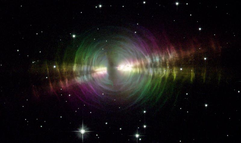
1) Rainbow image of a dusty star, NASA, http://hubblesite.org/newscenter/archive/releases/nebula/planetary/2003/09/

It's called the "Egg Nebula". You can see layers of dust coming out puff after puff, shooting outwards at about 20 kilometers per second, stretching out for about a third of a light year. The colors - red, green and blue - aren't anything you'd actually see. They're just an easy way to depict three different polarizations of light. I don't know why the light is polarized that way.

You can see a dark disk of thicker dust running around the star. It could be an "accretion disk" spiralling into the star. The "beams" shining out left and right are still poorly understood. Maybe they're jets of matter ejected from the north and south poles of the disk? This idea seem more plausible when you look at this photo taken by NICMOS, which is Hubble's "Near Infrared Camera and Multi-Object Spectrometer":

2) Raghvendra Sahai, Egg Nebula in polarized light, Hubble Heritage Project, http://heritage.stsci.edu/2003/09/supplemental.html

This near-infrared image also shows a bright spot called "Peak A" about 500 AU from the central star. An "AU", or astronomical unit, is the distance from the Sun to the Earth.

Nobody knows what this bright spot is. Some argue that it's just a clump of dust reflecting light from the main star. Others advocate a more exciting theory: it's a white dwarf orbiting the main star, which exploded in a "thermonuclear burst" after accreting a bunch of dust.

3) Joel H. Kastner and Noam Soker, The Egg Nebula (AFGL 2688): deepening enigma, to appear in Asymmetrical Planetary Nebulae III, eds. M. Meixner, J. Kastner, N. Soker, and B. Balick, ASP Conference Series. Available as arXiv:astro-ph/0309677.

I hope to say more about planetary nebulae in future Weeks, mainly because they're so beautiful.

But now: the field with one element!

A field is a mathematical structure where you can add, multiply, subtract and divide in ways that satisfy these familiar rules:

 x + y = y + x        (x + y) + z = x + (y + z)   x + 0 = x

 xy = yx              (xy)z = x(yz)               1x = x

 x(y + z) = xy + xz 

 every element x has an element -x with x + (-x) = 0
 
 every element x that's not 0 has an element 1/x with x (1/x) = 1

You'll note that the last clause is the odd man out. Addition, subtraction and multiplication can all be described as everywhere defined operations. Division cannot, since we can't divide by 0. This is the funny thing about fields, which is what causes the problem we'll run into.

Everyone who has studied math knows three examples of fields: the rational numbers Q, the real numbers R and the complex numbers C. There are a lot more, too - for example, function fields, number fields, and finite fields.

Let me say a tiny bit about these three kinds of fields.

The simplest sort of "function field" consists of rational functions of one variable - that is, ratios of polynomials, like this:

(2z³ + z + 1)/(z² - 7)

Here the coefficients of your polynomials should lie in some field F you already know about. The resulting field is called F(z). If F is the complex numbers, we can think of F(z) = C(z) as consisting of functions on the Riemann sphere. In "week201", I explained how the symmetries of this field form a group important in special relativity: the Lorentz group!

It's also very interesting to study the field of functions on a surface fancier than the sphere, but still defined by algebraic equations, like the surface of a doughnut or n-holed doughnut. Number theorists and algebraic geometers spend a lot of time thinking about these fields, which are called "function fields of complex curves".

For example, different ways of describing the surface of a doughnut by algebraic equations give different "elliptic curves". This is terminology is bound to puzzle beginners! They're called "curves" even though it's 2-dimensional, because it takes one complex number to say where you are on a little patch of a surface, just as it takes one real number to say where you are on an ordinary curve like a circle. That's the origin of the term "complex curve". And, they're called "elliptic" because they first showed up when people were studying elliptic integrals, which are generalizations of trig functions from circles to ellipses.

I explained more about elliptic curves in "week13" and "week125". Lurking behind this, there's a lot of fascinating stuff about function fields of elliptic curves.

The simplest sort of "number field" comes from taking the rational numbers and throwing in the solutions of a polynomial equation. For example, in "week20" I talked about the "golden field", which consists of all numbers of the form

a + b √ 5

where a and b are rational.

One of the most beautiful ideas in math is the analogy between number fields and function fields - the idea that numbers are like functions on some sort of "space". I began explaining this in "week205", "week216" and "week218", but there's much more to say about what's known... and also many things that remain mysterious.

In particular, it's pretty well understood how number fields resemble function fields of complex curves, and how this relates number theory to 2-dimensional topology. But, there are also many analogies between number theory and 3-dimensional topology, which I began listing in "week257". It seems these analogies are doomed to remain mysterious until we get a handle on the field with one element. But more on that later.

The simplest sort of "finite field" comes from choosing a prime number p and taking the integers modulo p. The result is sometimes called Z/p, especially when you're just concerned with addition. But when you think of it as a field, it's better to call it F_p.

The reason is that there's a finite field of size q whenever q is a power of a prime, and this field is unique - so it's called F_q. You build F_q sort of like how you build the complex numbers starting from the real numbers, or number fields starting from the rational numbers. Namely, to construct F_pⁿ, you take F_p and throw in the roots of a well-chosen polynomial of degree n: one that doesn't have any roots in F_p, but "wants" to have n different roots.

Okay: that was a tiny bit about function fields, number fields and finite fields. But now I need to point out some slight lies I told!

I said there was a finite field with q elements whenever q was a prime power. You might think this should include q = 1, since 1 is the zeroth power of any prime.

So, is there a field with one element?

If so, it must have 1 = 0. That doesn't violate the definition of a field that I gave you... does it? The definition said any element that's not 0 has a reciprocal. In this particular example, 0 also has a reciprocal, since we can set 1/0 = 1 and not get into any contradictions. But that's not a problem: in usual math practice, saying "we can divide by anything that's not zero" doesn't deny the possibility that we can divide by 0.

Unfortunately, allowing a field with 1 = 0 causes nothing but grief. For example, we can define vector spaces using any field (people say "over" any field), and there's a nice theorem saying two vector spaces are isomorphic if and only if they have the same dimension. And normally, there's one vector space of each dimension. But the last part isn't true for a field with 1 = 0. In a vector space over such a field, every vector v has

v = 1 v = 0 v = 0

So, every vector space is 0-dimensional!

To prevent such problems, people add one extra clause to the definition of a field:

 1 is not equal to 0

However, the field with one element still wants to exist! Not the silly field with 1 = 0, but something else, something more mysterious... something that Gavin Wraith calls a "mathematical phantom":

4) Gavin Wraith, Mathematical phantoms, http://www.wra1th.plus.com/gcw/rants/math/MathPhant.html

What's a mathematical phantom? According to Wraith, it's an object that doesn't exist within a given mathematical framework, but nonetheless "obtrudes its effects so convincingly that one is forced to concede a broader notion of existence".

Like a genie that talks its way out of a bottle, a sufficiently powerful mathematical phantom can talk us into letting it exist by promising to work wonders for us. Great examples include the number zero, irrational numbers, negative numbers, imaginary numbers, and quaternions. At one point all these were considered highly dubious entities. Now they're widely accepted. They "exist". Someday the field with one element will exist too!

Why?

I gave a lot of reasons in "week183", "week184", "week185", "week186" and "week187", but let me rapidly summarize.

It's all about "q-deformation". In physics, people talk about q-deformation when they're taking groups and turning them into "quantum groups". But it has a closely related aspect that's in some ways more fundamental. When we count things involving n-dimensional vector spaces over the finite field F_q, we often get answers that are polynomials in q. If we then set q = 1, the resulting formulas count analogous things involving n-element sets!

So, finite sets want to be finite-dimensional vector spaces over the (nonexistent) field with one element... or something like that. We can be more precise after looking at some examples.

Here's the simplest example. Say we count lines through the origin in an n-dimensional vector space over F_q. We get the "q-integer"

 qn - 1
------- = 1 + q + q2 + ... + qn-1
 q - 1

which I'll write as [n] for short.

Setting q = 1, we get n. This is the number of points in an n-element set. Sure, that sounds silly. But, I'm trying to make a point here! At q = 1, stuff about n-dimensional vector spaces over F_q reduces to stuff about n-element sets, and the q-integer [n] reduces to the ordinary integer n.

This may not be the best way to understand the pattern, though. Lines through the origin in an n-dimensional vector space are the same as points in an (n-1)-dimensional projective space. So, the real analogy may be between "points in a projective space" and "points in a set".

Here's a more impressive example. Pick any uncombed Young diagram D with n boxes. Here's one with 8 boxes:

X                     1 box in the first row
X X                   3 boxes in the first two rows
X X X                 6 boxes in the first three rows
X X                   8 boxes in the first four rows

    a 1-dimensional subspace
 of a 3-dimensional subspace
 of a 6-dimensional subspace
 of a 8-dimensional vector space over Fq

   a 1-element subset 
of a 3-element subset
of a 6-element subset
of a 8-element set

5) John Baez, Lecture 4 in the Geometric Representation Theory Seminar, October 9, 2007. Available at http://math.ucr.edu/home/baez/qg-fall2007/qg-fall2007.html#f07_4

These examples can be generalized. In "week187" I showed how to get one example for each subset of the dots in any Dynkin diagram! This idea goes back to Jacques Tits, who was the first to suggest that there should be a field with one element. Dynkin diagrams give algebraic groups over F_q... but he noticed that these groups reduce to "Coxeter groups" as q → 1. And, if you mark some dots on a Dynkin diagram you get a "flag variety" on which your algebraic group acts... but as q → 1, this reduces to a finite set on which your Coxeter group acts.

If you don't understand the previous paragraph, don't worry - it's over now. It's great stuff, but my main point is that there seems to be an analogy like this:

 q = 1                      q = a power of a prime number    

 n-element set              (n-1)-dimensional projective space over Fq
 integer n                  q-integer [n]
 permutation groups Sn      projective special linear group PSL(n,Fq)
 factorial n!               q-factorial [n]!

People have thought about this, and the answer seems to be "pointed sets" - sets with a distinguished point, which you can think of as the "origin". A pointed set with n+1 elements seems to act like an n-dimensional vector space over F_q.

For more clues, and an attempt to do algebraic geometry using the field with one element, try this:

6) Christophe Soulé, On the field with one element, Talk given at the Arbeitstagung, Bonn, June 1999, IHES preprint available at http://www.ihes.fr/~soule/f1-soule.pdf

Soulé tries to define "algebraic varieties" over F₁, namely curves and their higher-dimensional generalization. And, he talks a lot about zeta functions for such varieties. He goes into more detail here:

7) Christophe Soulé, Les varietes sur le corps a un element, Moscow Math. Jour. 4 (2004), 217-244, 312.

The theme of zeta functions - see "week216" - is deeply involved in this business. For more, try these papers:

8) N. Kurokawa, Zeta functions over F₁, Proc. Japan Acad. Ser. A Math. Sci. 81 (2006), 180-184.

9) Anton Deitmar, Remarks on zeta functions and K-theory over F₁, available as arXiv:math/0605429.

But instead of talking about zeta functions, I'd like to talk about two approaches to giving a formal definition of the field with one element. Both of them involve taking the concept of field and modifying it so it doesn't necessary involve the operation of addition. The first one, due to Deitmar, simply throws out addition! The second, due to Nikolai Durov, allows for a wide choice of operations - and thus a wide supply of "exotic fields".

For Deitmar's approach, try these:

10) Anton Deitmar, Schemes over F₁, available as arXiv:math/0404185.

F₁-schemes and toric varieties, available as arXiv:math/0608179.

The usual approach to fields treats fields as specially nice commutative rings. A "commutative ring" is a gadget where you can add and multiply, and these rules hold:

 x + y = y + x        (x + y) + z = x + (y + z)   x + 0 = x

 xy = yx              (xy)z = x(yz)               1x = x

 x(y + z) = xy + xz 

 every element x has an element -x with x + (-x) = 0

 xy = yx              (xy)z = x(yz)               1x = x

All this so far is quite trivial, but Deitmar makes a nice attempt at redoing algebraic geometry to include this field with one element. One reason to do this is to understand the mysterious 3-dimensional aspect of number theory.

To explain this, I need to say a bit about "schemes". In ordinary algebraic geometry, we turn commutative rings into spaces to think about them geometrically. I explained this back in "week199" and "week205", but let me review quickly, and go further:

We can think of elements of a commutative ring R as functions on certain space called the "spectrum" of R, Spec(R). This space has a topology, so we can also talk about functions that are defined, not on all of Spec(R), but just part of Spec(R) - namely some open set. Indeed, for each open set U in Spec(R), there's a commutative ring O(U) consisting of those functions defined on U. These commutative rings are related in nice ways:

1. If the open set V is smaller than U, we can restrict functions from U to V, getting a ring homomorphism O(U) → U(V)
2. If U is covered by a bunch of open sets U_i, and we have a function f_i in each O(U_i), such that f_i and f_j agree when restricted to the set U_i ∩ U_j, then there's a unique function f in O(U) that restricts to each of these functions f_i.

So, Spec(R) is not just a topological space, it's equipped with a sheaf of commutative rings. People call this a "ringed space".

Whenever we have a ringed space, we can ask if it comes from a commutative ring R in the way I just sketched. If so, we call it an "affine scheme". Affine schemes are just a fancy geometrical way of talking about commutative rings!

More interestingly, whenever we have a ringed space, we can ask if it's locally isomorphic to one coming from a commutative ring. In other words: does every point have a neighborhood that, as a ringed space, looks like Spec(R) for some commutative ring R? Or in other words: is our ringed space locally isomorphic to an affine scheme? If so, we call it a "scheme".

A classic example of a scheme that's not an affine scheme is the Riemann sphere. There aren't any rational functions defined on the whole Riemann sphere, except for constants - the rest all blow up somewhere. So, it's hopeless trying to think of the Riemann sphere as an affine scheme.

But, for any open set U in the Riemann sphere there's a commutative ring O(U) consisting of rational functions that are defined on U. So, the Riemann sphere becomes a ringed space. And, it's locally isomorphic to the complex plane, which is the affine scheme corresponding to the commutative ring of complex polynomials in one variable. So, the Riemann sphere is a scheme!

For more on schemes, try this nice introduction, which actually has lots of pictures:

11) David Eisenbud and Joe Harris, The Geometry of Schemes, Springer, Berlin, 2000.

Now, we can talk about schemes "over a field F", meaning that each commutative ring O(U) is also a vector space over F, in a well-behaved way, giving us a "sheaf of commutative rings over F". For example, the Riemann sphere is a scheme over C.

There's a secret 3-dimensional aspect to the affine scheme Spec(Z), where Z is the commutative ring of integers. As explained in the Addenda to "week257", we might understand this if we could see Spec(Z) as a scheme over the field with one element! For more, see this:

12) M. Kapranov and A. Smirnov, Cohomology determinants and reciprocity laws: number field case, available at http://wwwhomes.uni-bielefeld.de/triepe/F1.html

So, we really need a theory of schemes over the field with one element. The problem is, F₁ isn't really a field. In Deitmar's approach, it's just a commutative monoid.

So, let me sketch how Deitmar gets around this. In a nutshell, he takes advantage of the fact that a lot of basic algebraic geometry only requires multiplication, not addition!

He starts by defining a "commutative ring over F₁" to be simply a commutative monoid. The simplest example is F₁ itself.

Now, watch how he gets away with never using addition:

He defines an "ideal" in a commutative monoid R to be a subset I for which the product of something in I with anything in R again lies in I. He says an ideal P is "prime" if whenever a product of two elements in R is in P, at least one of them is in P.

He defines the "spectrum" Spec(R) of a commutative monoid R to be the set of its prime ideals. He gives this the "Zariski topology". That's the topology where the closed sets are the whole space, or any set of prime ideals that contain a given ideal.

He then shows how to get a sheaf of commutative monoids on Spec(R). He defines a "scheme" to be a space equipped with a sheaf of commutative monoids that's locally isomorphic to one of this sort.

If you know algebraic geometry, these definitions should seem very familiar. And if you don't, you can just replace the word "monoid" by "ring" everywhere in the previous three paragraphs, and you'll get the standard definitions in algebraic geometry!

Deitmar shows how to build a scheme over F₁ called the "projective line". The projective line over C is just the Riemann sphere. The projective line over F₁ has just two points (or more precisely, two closed points). This is good, because the projective line over the field with q elements has

[2] = 1 + q

points, and we're doing the q = 1 case.

Deitmar's construction seems like a lot of work to get ahold of the 2-element set, if that's all it secretly is. But, I need to think about this more. After all, he doesn't just get a space; he gets a sheaf of commutative monoids on this space! And what's that like? I should work it out.

Deitmar also shows how to relate schemes over F₁ to the usual sort of schemes.

From a commutative ring, we can always get a commutative monoid just by forgetting the addition. This process has a kind of reverse, too. Namely, from a commutative monoid, we can get a commutative ring simply by taking formal integral linear combinations of elements. Using this, Deitmar shows how we can turn ordinary schemes into schemes over F₁... and conversely. He says an ordinary scheme is "defined over F₁" if it arises in this way from a scheme over F₁.

Okay, that's a taste of Deitmar's approach. For Durov's approach, try this mammoth 568-page paper:

13) Nikolai Durov, New approach to Arakelov geometry, available as arXiv:0704.2030.

or read our discussions of it at the n-Category Café, starting here:

14) David Corfield, The field with one element, http://golem.ph.utexas.edu/category/2007/04/the_field_with_one_element.html

Durov defines a "generalized ring" to be what Lawvere much earlier called an "algebraic theory". What is it? Nothing scary! It's just a gadget with a bunch of abstract n-ary operations closed under composition, permutation, duplication and deletion of arguments, and equipped with an identity operation.

So, for example, if our gadget has a binary operation

(x,y) |→ f(x,y)

we can compose this with itself to get the ternary operation

(x,y,z) |→ f(f(x,y),z)

and the 4-ary operation

(w,x,y,z) |→ f(w,f(x,f(y,z)))

and so on. We can then permute arguments in our 4-ary operation to get one like this:

(w,x,y,z) |→ f(z,f(x,f(w,y)))

or duplicate some arguments to get a binary operation like this

(x,y) |→ f(x,f(x,f(y,y)))

From this we can then form a 3-ary operation by deleting an argument, for example like this:

(x,y,z) |→ f(x,f(x,f(y,y)))

If you know about "operads", this kind of gadget is just a specially nice operad where we can duplicate and delete operations.

Now, a generalized ring is said to be "commutative" if all the operations commute in a certain sense. (I'll let you guess what it means for an n-ary operation to commute with an m-ary operation.) We get an example of a commutative generalized ring from a commutative ring R if we let the n-ary operations be "n-ary R-linear combinations", like this:

(x₁, ..., x_n) |→ r₁ x₁ + ... + r_n x_n

We also get a very similar example from any commutative "rig", which is a gizmo satisfying rules like those of a commutative ring, but without negatives:

 x + y = y + x        (x + y) + z = x + (y + z)   x + 0 = x

 xy = yx              (xy)z = x(yz)               1x = x

 x(y + z) = xy + xz 

(x₁) |→ r x₁

So, Durov's framework generalizes Deitmar's! But, it includes a lot more examples: exotic hothouse flowers like the "tropical rig", the "real integers", and more. He develops a theory of schemes for all these generalized rings, and builds it "up to construction of algebraic K-theory, intersection theory and Chern classes" - fancy things that algebraic geometers like.

What I don't yet see is how either Deitmar's or Durov's approach helps us understand the secret 3-dimensional nature of Spec(Z). I may just need to read their papers more carefully and think about them more.

Finally, here's yet another approach to the field with one element:

15) Bertrand Toen and M. Vaquie, Under Spec(Z), available as arXiv:math/0509684.

16) Shai Haran, Non-additive geometry, Composito Mathematica 143 (2007), 613-638.

Toen describes interesting relations between algebra over F₁ and stable homotopy theory. Haran even suggests that the Riemann Hypothesis could be proved if we understood enough about the geometry of schemes over F₁! This is fascinating... I don't understand it, but I want to.

In short, a mathematical phantom is gradually taking solid form before our very eyes! In the process, a grand generalization of algebraic geometry is emerging, which enriches it to include some previously scorned entities: rigs, monoids and the like. And, this enrichment holds the promise of shedding light on some otherwise impenetrable mysteries: for example, the deep inner meaning of q-deformation, and the 3-dimensional nature of Spec(Z).

Addenda: I thank Thomas Riepe and David Corfield for drawing my attention to the paper by Shai Haran. Thomas Riepe also recommends the following online introduction to schemes:

17) Marc Levine, Summer course in motivic homotopy theory, available at http://www.math.neu.edu/~levine/publ/SummerSchoolAG.pdf

Kevin Buzzard has a word of advice about the "generic point":

  We can think of elements of a commutative ring R as functions on
  certain space called the "spectrum" of R, Spec(R).

So this is the set of all prime ideals of R, right? Not just the maximal ones? So...

  So, the Riemann sphere is a scheme!

Well, you have to throw in a mystical extra "generic point" if you really want to make it a scheme :-) Corresponding to the zero ideal. My impression is that most non-algebraic geometers think that the generic point is either confusing or just plain daft. But believe me, it's a really good idea! For decades in the literature in algebraic geometry people were using the word "generic" to mean "something that was true most of the time" - in fact a "generic point" is probably another really good example of a phantom! For example a meromorphic function on the Riemann sphere that wasn't zero would be "generically non-zero" to people like Borel and Weil, and if you asked them for a definition they would say that it just meant something like "the zero locus in the space had a smaller dimension than the whole space" or "the zero locus was nowhere dense in any component of the space" or something, and of course people could even make rigorous definitions that worked in particular cases and so on, but then Grothendieck came along with his "generic point", corresponding to the zero ideal [note to sub: check to see whether the idea was in the literature pre-Grothendieck!] and suddenly a function that was "generically non-zero" was just a function which was non-zero on the generic point! Such a cool way of doing it :-)

Kevin

If you get stuck on my puzzle "what does it mean for an n-ary operation to commute with an m-ary operation?", let me just show you what it means for a binary operation f to commute with a ternary operation g. It means:

g(f(x₁,x₂), f(x₃,x₄), f(x₅,x₆)) = f(g(x₁,x₂,x₃), g(x₄,x₅,x₆))

I hope this example gives away the general pattern.

If this is confusing, look at the case where we start with a ring R and take as our n-ary operations the "n-ary R-linear combinations"

(x₁, ..., x_n) |→ r₁ x₁ + ... + r_n x_n

with r_i in R. Here an example of a binary operation is addition:

(x₁, x₂) |→ x₁ + x₂

while every unary operation is multiplication by some element of R:

x₁ |→ r x₁

To say "addition commutes with multiplication by an element of R" means that

r(x₁ + x₂) = rx₁ + rx₂

This is just the distributive law so it holds for any ring R.

But, for the unary operations to commute with each other, we need R to be commutative, since this says:

r(s x₁) = s (r x₁)

(In the calculations I just did, we can either think of the x_i as elements of a specific R-module, or more abstractly as "dummy variables" used to describe the ring R as a generalized ring in Durov's sense - what Lawvere calls an algebraic theory.)

For more discussion, go to the n-Category Café.

© 2007 John Baez
baez@math.removethis.ucr.andthis.edu