3.4 The Route to Spin(10) via Pati-Salam
In the last section, we showed how the Pati-Salam model answers two questions
about the Standard Model:
Why are quarks and leptons so similar? Why are left and right so
different?
We were able to describe leptons as a fourth color of quark, `white', and
treat right-handed and left-handed particles on a more equal footing.
Neither of these ideas worked on its own, but together, they made
a full-fledged extension of the Standard Model, much like  and
and
 , but based on seemingly different principles.
Yet thinking of leptons as `white' should be strangely familiar, not
just from the Pati-Salam perspective, but
from the binary code that underlies both the and the
theories. There, leptons were indeed white: they all have
color
 .
.
Alas, while hints that leptons might be a fourth color, it does not
deliver on this. The quark colors
lie in a different irrep of than does
 . So, leptons in the theory are white, but unlike
the Pati-Salam model, this theory
does not unify leptons with quarks.
. So, leptons in the theory are white, but unlike
the Pati-Salam model, this theory
does not unify leptons with quarks.
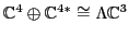
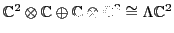
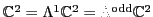
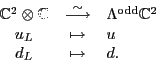
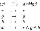
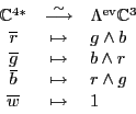
Yet theory is not the only game in town when it comes to the binary
code. We also have
, which acts on the same vector space as
. As a representation of
,
 breaks up into just
two irreps: the even grades,
breaks up into just
two irreps: the even grades,
 , which contain the left-handed
particles and antiparticles:
, which contain the left-handed
particles and antiparticles:
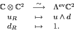
and the odd grades
 , which contain the right handed particles and
antiparticles:
, which contain the right handed particles and
antiparticles:
Unlike , the
GUT really does unify
 with the colors
  ,
,  and
and  , because they
both live in the irrep
.
, because they
both live in the irrep
.
In short, it seems that the
GUT, which we built as an
extension of the GUT, somehow managed to pick up
this feature of the Pati-Salam model.
How does
relate to Pati-Salam's gauge group
 ,
exactly? In general, we only know there is a map
,
exactly? In general, we only know there is a map
 ,
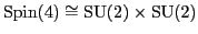
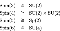
but in low dimensions, there is much more, because some groups coincide:
,
but in low dimensions, there is much more, because some groups coincide:
What really stands out is this:
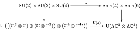
This brings out an obvious relationship between the Pati-Salam model and the
theory, because the inclusion
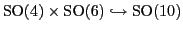 lifts to the universal covers, so we get a homomorphism
A word of caution is needed here. While  is the lift of an inclusion, it
is not an inclusion itself: it is two-to-one. This is because the universal
cover
is the lift of an inclusion, it
is not an inclusion itself: it is two-to-one. This is because the universal
cover
 of
of
 is a four-fold
cover, being a double cover on each factor.
is a four-fold
cover, being a double cover on each factor.
So we can try to extend the symmetries
to
, though this can only work if the kernel of acts
trivially on the Pati-Salam representation.
What is this representation like? There is an obvious
representation of
that extends to a
rep.
Both  and
and  have Dirac spinor representations, so their
product
has a representation on
have Dirac spinor representations, so their
product
has a representation on
 . And in fact, the obvious map
given by
is an isomorphism compatible with the actions of
on these two spaces. More concisely, this square:
commutes.
We will prove this in a moment. First though, we must check that
this representation of
is secretly
just another name for the Pati-Salam representation of
on the space we discussed in
Section 3.3:
Checking this involves choosing an isomorphism between
and
.
Luckily, we can choose one that works:
Theorem 4
.
There exists an isomorphism of Lie groups
and a unitary operator
that make this square commute:
where the left vertical arrow is the Pati-Salam representation
and the right one is a tensor product of Dirac spinor representations.
Proof. We can prove this in pieces, by separately finding
a unitary operator
that makes this square commute:
and a unitary operator
that make this square:
commute.
First, the piece. It suffices to show that the Dirac spinor rep
of
 on
on
 is isomorphic to
 as a rep of
 . We start with the action of on
. This breaks up
into irreps:
. We start with the action of on
. This breaks up
into irreps:
called the left-handed
and right-handed Weyl spinors, and these are dual to each
other because 6 = 2 mod 4, by a theorem that can be found
in Adams' lectures [1]. Call these representations
Since these reps are dual, it suffices just to consider one of them, say
 .
.
Passing to Lie algebras, we have a homomorphism
Homomorphic images of semisimple Lie algebras are semisimple, so the image of
 must lie entirely in
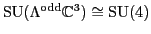
 . In fact
is simple, so this
nontrivial map must be an injection
. In fact
is simple, so this
nontrivial map must be an injection
and because the dimension is 15 on both sides, this map is also
onto. Thus
 is an isomorphism of Lie algebras, so
is an isomorphism of the simply connected Lie
groups and :
is an isomorphism of Lie algebras, so
is an isomorphism of the simply connected Lie
groups and :
Furthermore, under this isomorphism
as a representation of
 .
Taking duals, we obtain an isomorphism
.
Taking duals, we obtain an isomorphism
Putting these together, we get an isomorphism
 that makes this square commute:
which completes the proof for .
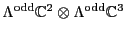
Next, the piece. It suffices
to show that the spinor rep
 of
of
 is isomorphic to
 as a rep of
 . We start with the action of on
. This
again breaks up into irreps:
. We start with the action of on
. This
again breaks up into irreps:
Again we call these representations
First consider
 . Passing to Lie algebras, this gives
a homomorphism
. Passing to Lie algebras, this gives
a homomorphism
Homomorphic images of semisimple Lie algebras are semisimple, so the image of
 must lie entirely in
 . Similarly,
also takes
to
:
. Similarly,
also takes
to
:
and we can combine these maps to get
which is just the derivative of 's representation on
.
Since this representation is faithful, the map
 of Lie
algebras is injective. But the dimensions of
and
of Lie
algebras is injective. But the dimensions of
and
 agree, so
is also onto. Thus it is an isomorphism
of Lie algebras. This implies that
agree, so
is also onto. Thus it is an isomorphism
of Lie algebras. This implies that
 is an isomorphism of of
the simply connected Lie groups and
is an isomorphism of of
the simply connected Lie groups and
under which
acts on
 . The
left factor of
. The
left factor of  acts irreducibly on
 , which the second
factor is trivial on. Thus
, which the second
factor is trivial on. Thus
 as a rep of
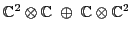
. Similarly,
as a rep of
. Similarly,
 as a rep of this group. Putting these together,
we get an isomorphism
as a rep of this group. Putting these together,
we get an isomorphism
 that makes this square commute:
which completes the proof for . 

In the proof of the preceding theorem, we merely showed that there
exists an isomorphism
making the square commute. We did not say exactly what  was.
In the proof, we built it after quietly choosing
three unitary operators, giving these isomorphisms:
was.
In the proof, we built it after quietly choosing
three unitary operators, giving these isomorphisms:
Since the remaining map
 is determined by
duality, these three operators determine , and they also
determine the Lie group isomorphism
is determined by
duality, these three operators determine , and they also
determine the Lie group isomorphism  via the construction in our proof.
There is, however, a specific choice for these unitary operators that we
prefer, because this choice makes the particles in the Pati-Salam
representation
look almost exactly like
those in the representation
.
First, since
 is spanned by
  and
and
 , the (left-handed) isospin states of the Standard Model, we really ought
to identify the left-isospin states
, the (left-handed) isospin states of the Standard Model, we really ought
to identify the left-isospin states  and
and  of the Pati-Salam model
with these. So, we should use this unitary operator:
of the Pati-Salam model
with these. So, we should use this unitary operator:
Next, we should use this unitary operator for right-isospin states:
Why? Because the right-isospin up particle is the right-handed neutrino
 , which corresponds to
 in the theory, but
  in the Pati-Salam model. This suggests that
  and
and  should be identified.
Finally, because
 is spanned by the colors , and , while
 is spanned by the colors , , and
  , we really ought
to use this unitary operator:
, we really ought
to use this unitary operator:
Dualizing this, we get the unitary operator
These choices determine the unitary operator
With this specific choice of , we can combine the commutative squares
built in Theorems 3 and
4:
to obtain the following result:
Theorem 5
.
Taking
 and
and  , the
following square commutes:
where the left vertical arrow is the Standard Model representation and
the right one is a tensor product of Dirac spinor representations.
, the
following square commutes:
where the left vertical arrow is the Standard Model representation and
the right one is a tensor product of Dirac spinor representations.
The map  , which tells us how to identify
  and
, is given by applying to the `Pati-Salam code' in
Table 5. This gives a binary code for the
Pati-Salam model:
and
, is given by applying to the `Pati-Salam code' in
Table 5. This gives a binary code for the
Pati-Salam model:
Table 6:
Pati-Salam binary code for first-generation fermions, where  and
and
 .
.
| The Binary Code for Pati-Salam |
 |
 |
 |
 |
 |
 |
 |
 |
 |
 |
 |
 |
 |
 |
 |
 |
 |
 |
 |
 |
|
We have omitted wedge product symbols to save space. Note that if we apply the
obvious isomorphism
given by
then the above table does more than
merely resemble Table 4, which gives the
binary code for the theory. The two tables become
identical!
This fact is quite intriguing. We will explore its meaning
in the next section. But first, let us start by relating the
Pati-Salam model to the
theory:
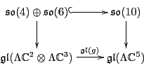
Theorem 6
.
The following square commutes:
where the right vertical arrow is the Dirac spinor representation,
the left one is the tensor product of Dirac spinor representations,
and
is the homomorphism lifting the inclusion of
in
 .
.
Proof. At the Lie algebra level, we have the inclusion
by block diagonals, which is also just the differential of the inclusion
at the Lie group level. Given how the
spinor reps are defined in terms of creation and annihilation operators, it is
easy to see that
commutes, because is an
intertwining operator between representations
of
 .
That is because the
part only acts on
, while the
part only acts on
.
.
That is because the
part only acts on
, while the
part only acts on
.
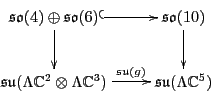
But these Lie algebras act by skew-adjoint operators, so really
commutes. Since the
 's and their direct sums are semisimple, so are
their images. Therefore, their images live in the semisimple part of the
unitary Lie algebras, which is just another way of saying the special unitary
Lie algebras. We get that
's and their direct sums are semisimple, so are
their images. Therefore, their images live in the semisimple part of the
unitary Lie algebras, which is just another way of saying the special unitary
Lie algebras. We get that
commutes, and this gives a commutative square in the world of
simply connected Lie groups:
This completes the proof.
This result shows us how to reach the
theory, not
through the theory, but through the Pati-Salam model.
For physics texts that treat this issue, see for example
Zee [40] and Ross [31].
2010-01-11
![\begin{displaymath}
\xymatrix{
{\rm Spin}(4) \times {\rm Spin}(6) \ar[r]^-\eta \...
...3) \ar[r]^-{{\rm U}(g)} & {\rm U}(\Lambda {\mathbb C}^5) \\
}
\end{displaymath}](img661.png)
![\begin{displaymath}
\xymatrix{
{\rm SU}(2) \times {\rm SU}(2) \ar[r]^-\sim \ar[d...
...thbb C}^2) \ar[r]^-\sim & {\rm U}(\Lambda {\mathbb C}^2) \\
}
\end{displaymath}](img667.png)
![\begin{displaymath}
\xymatrix{
{\rm SU}(4) \ar[r]^\sim \ar[d] & {\rm Spin}(6) \a...
...b C}^{4*}) \ar[r]^-\sim & {\rm U}(\Lambda {\mathbb C}^3) \\
}
\end{displaymath}](img669.png)
![\begin{displaymath}
\xymatrix{
{\rm Spin}(6) \ar[d] \ar[r]^\rho_{\rm{odd}}& {\rm...
...}^3) \ar[r] & {\rm U}({\mathbb C}^4 \oplus {\mathbb C}^{4*})
}
\end{displaymath}](img684.png)
![\begin{displaymath}
\xymatrix{
{\rm Spin}(4) \ar[d] \ar[r]^-{\rho_{\rm{ev}}\oplu...
... \otimes {\mathbb C}\oplus {\mathbb C}\otimes {\mathbb C}^2)
}
\end{displaymath}](img704.png)
![\begin{displaymath}
\xymatrix{
{G_{\mbox{\rm SM}}}\ar[r]^-{\beta} \ar[d]
& {\rm...
...ght) \ar[r]^-{{\rm U}(k)}
& {\rm U}(\Lambda {\mathbb C}^5)
}
\end{displaymath}](img716.png)
![\begin{displaymath}
\xymatrix{
{G_{\mbox{\rm SM}}}\ar[r]^-\theta \ar[d] & {\rm...
...}(\Lambda {\mathbb C}^2 \otimes \Lambda {\mathbb C}^3) \\
}
\end{displaymath}](img719.png)
![\begin{displaymath}
\xymatrix{
{\mathfrak{so}}(4) \oplus {\mathfrak{so}}(6) \ar@...
...thbb C}^3) \ar[r]^-{\u (g)} & \u (\Lambda {\mathbb C}^5) \\
}
\end{displaymath}](img744.png)
![\begin{displaymath}
\xymatrix{
{\rm Spin}(4) \times {\rm Spin}(6) \ar[r]^-\eta \...
...}^3) \ar[r]^-{{\rm SU}(g)} & {\rm SU}(\Lambda {\mathbb C}^5)
}
\end{displaymath}](img747.png)