Warming Slowdown?

Jan Galkowski
Akamai Technologies
empirical_bayesian@ieee.org
Cambridge, MA 02142
18^th May 2014
	(revised draft 007, HTML version)

1. How Heat Flows and Why It Matters

Is there something missing in the recent climate temperature record?

Heat is most often experienced as energy density, related to temperature. While technically temperature is only meaningful for a body in thermal equilibrium, temperature is the operational definition of heat content, both in daily life and as a scientific measurement, whether at a point or averaged. For the present discussion, it is taken as given that increasing atmospheric concentrations of carbon dioxide trap and re-radiate Earth blackbody radiation to its surface, resulting in a higher mean blackbody equilibration temperature for the planet, via radiative forcing [Ca2014a, Pi2012, Pi2011, Pe2006]. The question is, how does a given Joule of energy travel? Once on Earth, does it remain in atmosphere? Warm the surface? Go into the oceans? And, especially, if it does go into the oceans, what is its residence time before released to atmosphere? These are important questions [Le2012a, Le2012b]. Because of the miscibility of energy, questions of residence time are very difficult to answer. A Joule of energy can't be tagged with a radioisotope like matter sometimes can. In practice, energy content is estimated as a constant plus the time integral of energy flux across a well-defined boundary using a baseline moment.

Variability is a key aspect of natural systems, whether biological or large scale geophysical systems such as Earth's climate [Sm2009]. Variability is also a feature of statistical models used to describe behavior of natural systems, whether they be straightforward empirical models or models based upon ab initio physical calculations. Some of the variability in models captures the variability of the natural systems which they describe, but some variability is inherent in the mechanism of the models, an artificial variability which is not present in the phenomena they describe. No doubt, there is always some variability in natural phenomena which no model captures. This variability can be partitioned into parts, at the risk of specifying components which are not directly observable. Sometimes they can be inferred.

Models of planetary climate are both surprisingly robust and understood well enough that appreciable simplifications, such as setting aside fluid dynamism, are possible, without damaging their utility [Pi2012]. Thus, the general outline of what long term or asymptotic and global consequences arise when atmospheric carbon dioxide concentrations double or triple are known pretty well. More is known from the paleoclimate record. What is less certain are the dissipation and diffusion mechanisms for this excess energy and its behavior in time [Kr2014, Sh2014a, Sh2014b, Sa2011]. There is keen interest in these mechanisms because of the implications differing magnitudes have for regional climate forecasts and economies [Em2011, Sm2011, Le2010]. Moreover, there is a natural desire to obtain empirical confirmation of physical calculations, as difficult as that might be, and as subjective as judgments regarding quality of predictions might be [Sc2014, Be2013, Mu2013a, Mu2013b, Br2006, Co2013, Fy2013, Ha2013, Ha2014, Ka2013a, Sl2013, Tr2013, Mo2012, Sa2012, Ke2011a, Kh2008a, Kh2008b, Le2005, De1982].

Observed rates of surface temperatures in recent decades have shown a moderating slope compared with both long term statistical trends and climate model projections [En2014, Fy2014, Sc2014, Ta2013, Tr2013, Mu2013b, Fy2013, Fy2013s, Be2013]. It's the purpose of this article to present this evidence, and report the research literature's consensus on where the heat resulting from radiative forcing is going, as well as sketch some implications of that containment.

2. Tools of the Trade

I'm Jan Galkowski. I'm a statistician and signals engineer, with an undergraduate degree in Physics and a Masters in EE & Computer Science. I work for Akamai Technologies of Cambridge, MA, where I study time series of Internet activity and other data sources, doing data analysis primarily using spectral and Bayesian computational methods. I am not a climate scientist, but am keenly interested in the mechanics of oceans, atmosphere, and climate disruption. I approach these problems from that of a statistician and physical dynamicist. Climate science is an avocation. While I have 32 years experience doing quantitative analysis, primarily in industry, I have found that the statistical and mathematical problems I encounter at Akamai have remarkable parallels to those in some geophysics, such as hydrology and assessments of sea level rise, as well as in some population biology. Thus, it pays to read their literature and understand their techniques. I also like to think that Akamai has something significant to contribute to this problem of mitigating forcings of climate change, such as enabling and supporting the ability of people to attend business and science meetings by high quality video call rather than hopping on CO₂-emitting vehicles.

Finally, as the great J. W. Tukey said:

The best thing about being a statistician is that you get to play in everyone's backyard.

Anyone who doubts the fun of doing so, or how statistics enables such, should read Young.

3. On Surface Temperatures, Land and Ocean

Independently of climate change, monitoring surface temperatures globally is a useful geophysical project. They are accessible, can be measured in a number of ways, permit calibration and cross-checking, are taken at convenient boundaries between land-atmosphere or ocean-atmosphere, and coincide with the living space about which we most care. Nevertheless, like any large observational effort in the field, such measurements need careful assessment and processing before they can be properly interpreted. The Berkeley Earth Surface Temperature ("BEST") Project represents the most comprehensive such effort, but it was not possible without many predecessors, such as HadCRUT4, and works by Kennedy, et al and Rohde [Ro2013a, Mo2012, Ke2011a, Ke2011b, Ro2013b].

Surface temperature is a manifestation of four interacting processes. First, there is warming of the surface by the atmosphere. Second, there is lateral heating by atmospheric convection and latent heat in water vapor. Third, during daytime, there is warming of the surface by the Sun or insolation which survives reflection. Last, there is warming of the surface from below, either latent heat stored subsurface, or geologic processes. Roughly speaking, these are ordered from most important to least. These are all manifestations of energy flows, a consequence of equalization of different contributions of energy to Earth.

Physically speaking, the total energy of the Earth climate system is a constant plus the time integral of energy of non-reflected insolation less the energy of the long wave radiation or blackbody radiation which passes from Earth out to space, plus geothermal energy ultimately due to radioisotope decay within Earth's aesthenosphere and mantle, plus thermal energy generated by solid Earth and ocean tides, plus waste heat from anthropogenic combustion and power sources [Decay]. The amount of non-reflected insolation depends upon albedo, which itself slowly varies. The amount of long wave radiation leaving Earth for space depends upon the amount of water aloft, by amounts and types of greenhouse gases, and other factors. Our understanding of this has improved rapidly, as can be seen by contrasting Kiehl, et al in 1997 with Trenberth, et al in 2009 and the IPCC's 2013 WG1 Report [Ki1997, Tr2009, IP2013]. Steve Easterbrook has given a nice summary of radiative forcing at his blog, as well as provided a succinct recap of the 2013 IPCC WG1 Report and its take on energy flows elsewhere at the The Azimuth blog. I refer the reader to those references for information about energy budgets, what we know about them, and what we do not.

Some ask whether or not there is a physical science basis for the "moderation" in global surface temperatures and, if there is, how that might work. It is an interesting question, for such a conclusion is predicated upon observed temperature series being calibrated and used correctly, and, further, upon insufficient precision in climate model predictions, whether simply perceived or actual. Hypothetically, it could be that the temperature models are not being used correctly and the models are correct, and which evidence we choose to believe depends upon our short-term goals. Surely, from a scientific perspective, what's wanted is a reconciliation of both, and that is where many climate scientists invest their efforts. This is also an interesting question because it is, at its root, a statistical one, namely, how do we know which model is better [Ve2012, Sm2009, Sl2013, Ge1998, Co2006, Fe2011b, Bu2002]?

A first graph, Figure 1, depicting evidence of warming is, to me, quite remarkable.

Figure 1. Ocean temperatures at depth, from http://www.yaleclimatemediaforum.org/2013/09/examining-the-recent-slow-down-in-global-warming/.

A similar graph is shown in the important series recapping the recent IPCC Report by Steve Easterbrook. A great deal excess heat is going into the oceans. In fact, most of it is, and there is an especially significant amount going deep into the southern oceans, something which may have implications for Antarctica.

This can happen in many ways, but one dramatic way is due to a phase of the El Niño Southern Oscillation} ("ENSO"). Another way is storage by the Atlantic Meridional Overturning Circulation ("AMOC") [Ko2014].

The trade winds along the Pacific equatorial region vary in strength. When they are weak, the phenomenon called El Niño is seen, affecting weather in the United States and in Asia. Evidence for El Niño includes elevated sea-surface temperatures ("SSTs") in the eastern Pacific. This short-term climate variation brings increased rainfall to the southern United States and Peru, and drought to east Asia and Australia, often triggering

Figure 2. Oblique view of variability of Pacific equatorial region from El Niño to La Niña and back. Vertical height of ocean is exaggerated to show piling up of waters in the Pacific warm pool.

large wildfires there. The reverse phenomenon, La Niña, is produced by strong trades, and results in cold SSTs in the eastern Pacific, and plentiful rainfall in east Asia and northern Australia. Strong trades actually pile ocean water up against Asia, and these warmer-than-average waters push surface waters there down, creating a cycle of returning cold waters back to the eastern Pacific. This process is depicted in Figures 2 and 3.

Figure 3. Trade winds vary in strength, having consequences for pooling and flow of Pacific waters and sea surface temperatures.

At its peak, a La Niña causes waters to accumulate in the Pacific warm pool, and this results in surface heat being pushed into the deep ocean. To the degree to which heat goes into the deep ocean, it is not available in atmosphere. To the degree to which the trades do not pile waters into the Pacific warm pool and, ultimately, into the depths, that warm water is in contact with atmosphere [Me2011]. There are suggestions warm waters

Figure 4. Strong trade winds cause the warm surface waters of the equatorial Pacific to pile up against Asia.

at depth rise to the surface [Me2013].

Documentation of land and ocean surface temperatures is done in variety of ways. There are several important sources, including Berkeley Earth, NASA GISS, and the Hadley Centre/Climatic Research Unit ("CRU") data sets [Ro2013a, Ha2010, Mo2012] The three, referenced here as BEST, GISS, and HadCRUT4, respectively, have been compared by Rohde. They differ in duration and extent of coverage, but allow comparable inferences. For example, a linear regression establishing a trend using July monthly average temperatures from 1880 to 2012 for Moscow from GISS and BEST agree that Moscow's July 2010 heat was 3.67 standard deviations from the long term trend [GISS-BEST]. Nevertheless, there is an important difference between BEST and GISS, on the one hand, and HadCRUT4.

BEST and GISS attempt to capture and convey a single best estimate of temperatures on Earth's surface, and attach an uncertainty measure to each number. Sometimes, because of absence of measurements or equipment failures, there are no measurements, and these are clearly marked in the series. HadCRUT4 is different. With HadCRUT4 the uncertainty in measurements is described by a hundred member ensemble of values, actually a 2592-by-1967 matrix. Rows correspond to observations from 2592 patches, 36 in latitude, and 72 in longitude, with which it represents the surface of Earth. Columns correspond to each month from January 1850 to November 2013. It is possible for any one of these cells to be coded as "missing". This detail is important because HadCRUT4 is the basis for a paper suggesting the pause in global warming is structurally inconsistent with climate models. That paper will be discussed later.

4. Rumors of Pause

Figure 5 shows the global mean surface temperature anomalies relative to a standard baseline, 1950-1980. Before going on, consider that figure. Study it. What can you see in it?

Figure 5. Global surface temperature anomalies relative to a 1950-1980 baseline.

Figure 6 shows the same graph, but now with two trendlines obtained by applying a smoothing spline, one smoothing more than another. One of the two indicates an uninterrupted uptrend. The other shows a peak and a downtrend, along with wiggles around the other trendline. Note the smoothing algorithm is the same in both cases, differing only in the setting of

Figure 6. Global surface temperature anomalies relative to a 1950-1980 baseline, with two smoothing splines printed atop.

a smoothing parameter. Which is correct? What is "correct"?

Figure 7 shows a time series of anomalies for

Figure 7. Temperature anomalies for Moscow, Russia.

Moscow, in Russia. Do these all show the same trends? These are difficult questions, but the changes seen in Figure 6 could be evidence of a warming "hiatus". Note that, given Figure 6 whether or not there is a reduction in the rate of temperature increase depends upon the choice of a smoothing parameter. In a sense, that's like having a major conclusion depend upon a choice of coordinate system, something we've collectively learned to suspect. We'll have a more careful look at this in Section 5. With that said, people have sought reasons and assessments of how important this phenomenon is. The answers have ranged from the conclusive "Global warming has stopped" to "Perhaps the slowdown is due to 'natural variability"', to "Perhaps it's all due to "natural variability" to "There is no statistically significant change". Let's see what some of the perspectives are.

It is hard to find a scientific paper which advances the proposal that climate might be or might have been cooling in recent history. The earliest I can find are repeated presentations by a single geologist in the proceedings of the Geological Society of America, a conference which, like many, gives papers limited peer review [Ea2000, Ea2000, Ea2001, Ea2005, Ea2006a, Ea2006b, Ea2007, Ea2008]. It is difficult to comment on this work since their full methods are not available for review. The content of the abstracts appear to ignore the possibility of lagged response in any physical system.

These claims were summarized by Easterling and Wehner in 2009, attributing claims of a "pause" to cherry-picking of sections of the temperature time series, such as 1998-2008, and what might be called media amplification. Further, technical inconsistencies within the scientific enterprise, perfectly normal in its deployment and management of new methods and devices for measurement, have been highlighted and abused to parlay claims of global cooling [Wi2007, Ra2006, Pi2006]. Based upon subsequent papers, climate science seemed to not only need to explain such variability, but also to provide a specific explanation for what could be seen as a recent moderation in the abrupt warming of the mid-late 1990s. When such explanations were provided, appealing to oceanic capture, as described in Section 3, the explanation seemed to be taken as an acknowledge of a need and problem, when often they were provided in good faith, as explanation and teaching [Me2011, Tr2013, En2014].

Other factors besides the overwhelming one of oceanic capture contribute as well. If there is a great deal of melting in the polar regions, this process captures heat from the oceans. Evaporation captures heat in water. No doubt these return, due to the water cycle and latent heat of water, but the point is there is much opportunity for transfer of radiative forcing and carrying it appreciable distances.

Note that, given the overall temperature anomaly series, such as Figure 6, and specific series, such as the one for Moscow in Figure 7, moderation in warming is not definitive. It is a statistical question, and, pretending for the moment we know nothing of geophysics, a difficult one. But there certainly is no any problem with accounting for the Earth's energy budget overall, even if the distribution of energy over its surface cannot be specifically explained [Ki1997, Tr2009, Pi2012]. This is not a surprise, since the equipartition theorem of physics fails to apply to a system which has not achieved thermal equilibrium.

An interesting discrepancy is presented in a pair of papers in 2013 and 2014. The first, by Fyfe, Gillet, and Zwiers, has the (somewhat provocative) title "Overestimated global warming over the past 20 years". (Supplemental material is also available and is important to understand their argument.) It has been followed by additional correspondence from Fyfe and Gillet ("Recent observed and simulated warming") applying the same methods to argue that even with the Pacific surface temperature anomalies and explicitly accommodating the coverage bias in the HadCRUT4 dataset, as emphasized by Kosaka and Xie there remain discrepancies between the surface temperature record and climate model ensemble runs. In addition, Fyfe and Gillet dismiss the problems of coverage cited by by Cowtan and Way, arguing they were making "like for life" comparisons which are robust given the dataset and the region examined with CMIP5 models. How these scientific discussions present that challenge and its possible significance is a story of trends, of variability, and hopefully of what all these investigations are saying in common, including the important contribution of climate models.

5. Trends Are Tricky

Trends as a concept are easy. But trends as objective measures are slippery. Consider the Keeling Curve, the record of atmospheric carbon dioxide concentration first begun by Charles Keeling in the 1950s and continued in the face of great obstacles. This curve is reproduced in Figure 8, and there presented in its original, and then decomposed into three parts, an annual sinusoidal variation, a linear trend, and a stochastic remainder.

Figure 8. Keeling CO₂ concentration curve at Mauna Loa, Hawaii, showing original data and its decomposition into three parts, a sinusoidal annual variation, a linear trend, and a stochastic residual.

The question is, which component represents the true trend, long term or otherwise? Are linear trends superior to all others? The importance of a trend is tied up with to what use it will be put. A pair of trends, like the sinusoidal and the random residual of the Keeling, might be more important for predicting its short term movements. On the other hand, explicating the long term behavior of the system being measured might feature the large scale linear trend, with the seasonal trend and random variations being but distractions.

Consider the global surface temperature anomalies of Figure 5 again. What are some ways of determining trends? First, note that by "trends" what's really meant are slopes. In the case where there are many places to estimate slopes, there are many slopes. When, for example, a slope is estimated by fitting a line to all the points, there's just a single slope such as in Figure 9. Local linear trends can be estimated from pairs of points in differing sizes of neighborhoods, as depicted in Figures 10 and 11. These

Figure 9. Global surface temperature anomalies relative to a 1950-1980 baseline, with long term linear trend atop.

Figure 10. Global surface temperature anomalies relative to a 1950-1980 baseline, with randomly placed trends from local linear having 5 year support atop.

Figure 11. Global surface temperature anomalies relative to a 1950-1980 baseline, with randomly placed trends from local linear having 10 year support atop.

can be averaged, if you like, to obtain an overall trend. Lest the reader think constructing lots of linear trends on varying neighborhoods is somehow crude, note it has a noble history, being used by Boscovich to estimate Earth's ellipticity about 1750, as reported by Koenker.

There is, in addition, a question of what to do if local intervals for fitting the little lines overlap, since these are then (on the face of it) not independent of one another. There are a number of statistical devices for making them independent. One way is to do clever kinds of random sampling from a population of linear trends. Another way is to shrink the intervals until they are infinitesimally small, and, so, necessarily independent. That definition is just the point slope of a curve going through the data, or its first derivative. Numerical methods exist of estimating these, and to the degree they succeed, they obtain estimates of the derivative, even if in doing do they might use finite intervals. One good way of estimating derivatives involves using a smoothing spline, as sketched in Figure 6, and estimating the derivative(s) of that. Such an estimate of the derivative is shown in Figure 12 where the instantaneous slope is plotted in orange atop the data of Figure 6. The value of the derivative should be read using the scale to the right of the graph. The value to the left shows, as before, temperature anomaly in degrees. The cubic spline itself is plotted in green in that figure. Here it's smoothing parameter is determined by generalized cross-validation, a principled means of taking the subjectivity out of the choice of smoothing parameter. That is explained a bit more in the caption for Figure 12. (See also Cr1979.)

Figure 12. Global surface temperature anomalies relative to a 1950-1980 baseline, with instaneous numerical estimates of derivatives in orange atop, with scale for the derivative to the right of the chart. Note how the value of the first derivative *never drops below zero* although its *magnitude* decreases as time approaches 2012. Support for the smoothing spline used to calculate the derivatives is obtained using *generalized cross validation*. Such cross validation is used to help reduce the possibility that a smoothing parameter is chosen to *overfit* a particular data set, so the analyst could expect that the spline would apply to as yet uncollected data more than otherwise. Generalized cross validation is a particular clever way of doing that, although it is abstract.

What else might we do?

We could go after a really good approximation to the data of Figure 5. One possibility is to use the Bayesian Rauch-Tung-Striebel ("RTS") smoother to get a good approximation for the underlying curve and estimate the derivatives of that. This is a modification of the famous Kalman filter, the workhorse of much controls engineering and signals work. What that means and how these work is described in an accompanying inset box.

Using the RTS smoother demands variances of the signal be estimated as priors. The larger the ratio of the estimate of the observations variance to the estimate of the process variance is, the smoother the RTS solution. And, yes, as the reader may have guessed, that makes the result dependent upon initial conditions, although hopefully educated initial conditions.

Figure 13. Global surface temperature anomalies relative to a 1950-1980 baseline, with fits using the Rauch-Tung-Striebel smoother placed atop, in green and dark green. The former uses a prior variance of 3 times that of the Figure 5 data corrected for serial correlation. The latter uses a prior variance of 15 times that of the Figure 5 data corrected for serial correlation. The instantaneous numerical estimates of the first derivative derived from the two solutions are shown in orange and brown, respectively, with their scale of values on the right hand side of the chart. Note the two solutions are essentially identical. If compared to the smoothing spline estimate of Figure 12, the derivative has roughly the same shape, but is shifted lower in overall slope, and the drift up and below a mean value is less.

The RTS smoother result for two process variance values of 0.118 ± 002 and high 0.59 ± 0.02 is shown in Figure 13. These are 3 and 15 times the decorrelated variance value for the series of 0.039 ± 0.001, estimated using the long term variance for this series and others like it, corrected for serial correlation. One reason for using two estimates of the process variance is to see how much difference that makes. As carn be seen from Figure 13, it does not make much.

Combining all six methods of estimating trends results in Figure 14 which shows the overprinted densities of slopes.

Figure 14. Empirical probability density functions for slopes of temperatures versus years, from each of 6 methods. Empirical probability densities are obtained using kernel density estimation and are preferred to histograms by statisticians because the latter can distort the density due to bin size and boundary effects. Lines correspond to local linear fits with 5 years separation (dark green trace), the local linear fits with 10 years separation (green trace), the smoothing spline (blue trace), the RTS smoother with variance 3 times the corrected estimate for the data as the prior variance (orange trace, mostly hidden by brown trace), and the RTS smoother with 15 times the corrected estimate for the data (brown trace). The blue trace can barely be seen because the RTS smoother with the 3 times variance lies nearly atop of it. The slope value for a linear fit to all the points is also shown (the vertical black line).

Note the spread of possibilities given by the 5 year local linear fits. The 10 year local linear fits, the spline, and the RTS smoother fits have their mode in the vicinity of the overall slope. The 10 year local linear fits slope has broader support, meaning it admits more negative slopes in the range of temperature anomalies observed. The RTS smoother results have peaks slightly below those for the spline, the 10 year local linear fits, and the overall slope. The kernel density estimator allows the possibility of probability mass below zero, even though the spline, and two RTS smoother fits never exhibit slopes below zero. This is a Bayesian-like estimator, since the prior is the real line.

Local linear fits to HadCRUT4 time series were used by Fyfe, Gillet, and Zwiers in their 2013 paper and supplement. We do not know the computational details of those trends, since they were not published, possibly due to Nature Climate Change page count restrictions. Those details matter. From these calculations, which, admittedly, are not as comprehensive as those by Fyfe, Gillet, and Zwiers, we see that robust estimators of trends in temperature during the observational record show these are always positive, even if the magnitudes vary. The RTS smoother solutions suggest slopes in recent years are near zero, providing a basis for questioning whether or not there is a warming "hiatus".

The Rauch-Tung-Striebel smoother is an enhancement of the Kalman filter. Let $$y_{\kappa}$$ denote a set of univariate observations at equally space and successive time steps $$\kappa$$. Describe these as follows:

$$ y_{\kappa} = \mathbf{G} \mathbf{x}_{\kappa} + \varepsilon_{\kappa} $$
$$ \mathbf{x}_{\kappa + 1} = \mathbf{H} \mathbf{x}_{\kappa} + \boldsymbol\gimel_{\kappa} $$
$$ \varepsilon_{\kappa} \sim \mathcal{N}(0, \sigma^{2}_{\varepsilon}) $$
$$ \boldsymbol\gimel_{\kappa} \sim \mathcal{N}(0, \boldsymbol\Sigma^{2}_{\eta}) $$

The multivariate $$\mathbf{x}_{\kappa}$$ is called a state vector for index $$\kappa$$. $$\mathbf{G}$$ and $$\mathbf{H}$$ are given, constant matrices. Equations (5.3) and (5.4) say that the noise component of observations and states are distributed as zero mean Gaussian random variables with variance $$\sigma^{2}_{\varepsilon}$$ and covariance $$\boldsymbol\Sigma^{2}_{\eta}$$, respectively. This simple formulation in practice has great descriptive power, and is widely used in engineering and data analysis. For instance, it is possible to cast autoregressive moving average models ("ARMA") in this form. (See Kitigawa, Chapter 10.) The key idea is that equation (5.1) describes at observation at time $$\kappa$$ as the result of a linear regression on coefficients $$\mathbf{x}_{\kappa}$$, where $$\mathbf{G}$$ is the corresponding design matrix. Then, the coefficients themselves change with time, using a Markov-like development, a linear regression of the upcoming set of coefficients, $$\mathbf{x}_{\kappa+1}$$, in terms of the current coefficients, $$\mathbf{x}_{\kappa}$$, where $$\mathbf{H}$$ is the design matrix.

For the purposes here, a simple version of this is used, something called a local level model (Chapter 2) and occasionally a Gaussian random walk with noise model (Section 12.3.1). In that instance, $$\mathbf{G}$$ and $$\mathbf{H}$$ are not only scalars, they are unity, resulting in the simpler

$$ y_{\kappa} &= x_{\kappa} + \varepsilon_{\kappa} $$
$$ x_{\kappa + 1} &= x_{\kappa} + \eta_{\kappa} $$
$$ \varepsilon_{\kappa} &\sim \mathcal{N}(0, \sigma^{2}_{\varepsilon}) $$
$$ \eta_{\kappa} &\sim \mathcal{N}(0, \sigma^{2}_{\eta}) $$

with scalar variances $$\sigma^{2}_{\varepsilon}$$ and $$\sigma^{2}_{\eta}$$.

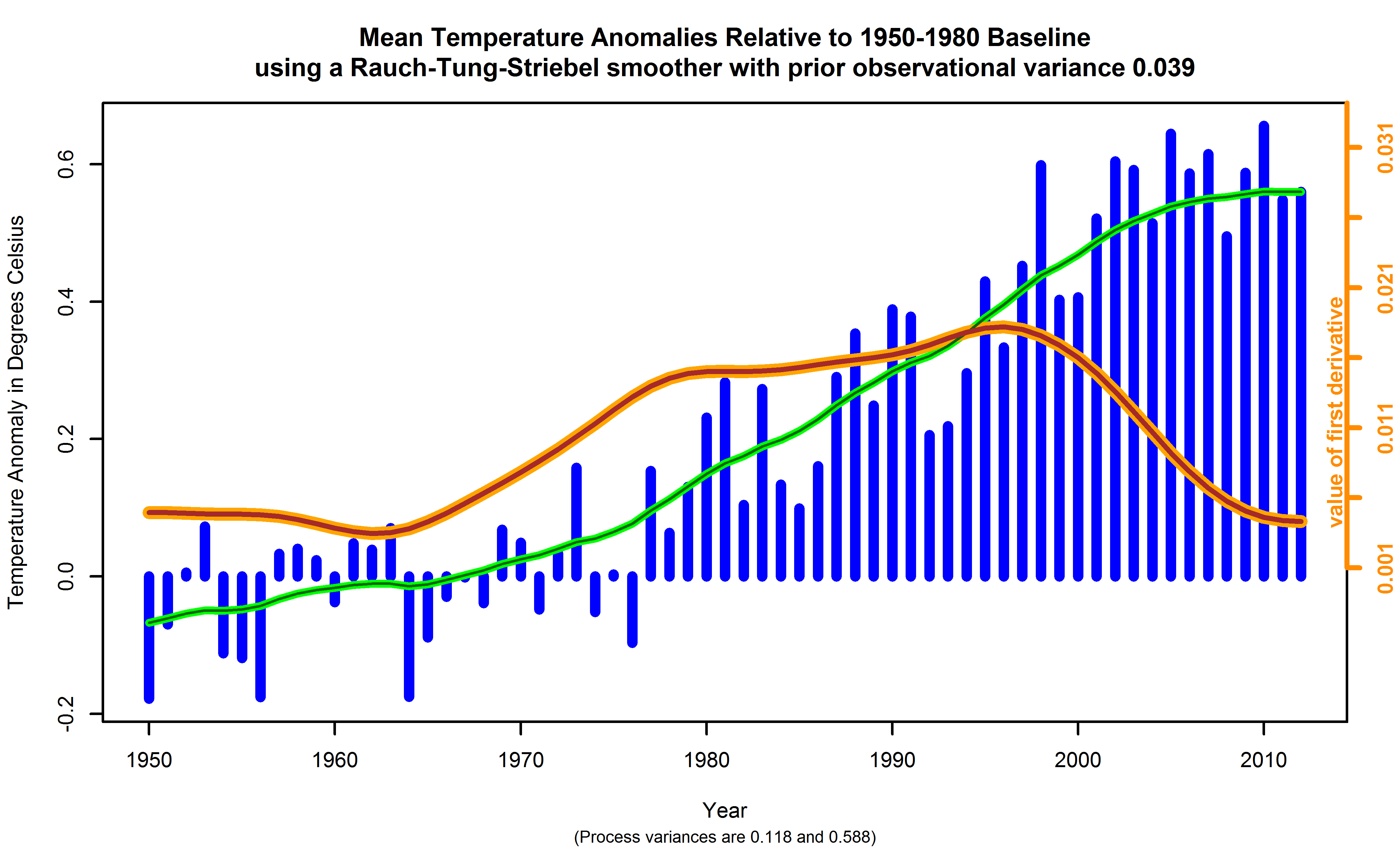
In either case, the Kalman filter is a way of calculating $$\mathbf{x}_{\kappa}$$, given $$y_{1}, y_{2}, \dots, y_{n}$$, values for $$\mathbf{G}$$ and $$\mathbf{H}$$, and estimates for $$\sigma^{2}_{\varepsilon}$$ and $$\sigma^{2}_{\eta}$$. Choices for $$\mathbf{G}$$ and $$\mathbf{H}$$ are considered a model for the data. Choices for $$\sigma^{2}_{\varepsilon}$$ and $$\sigma^{2}_{\eta}$$ are based upon experience with $$Y_{\kappa}$$ and the model. In practice, and within limits, the bigger the ratio

$$\frac{\sigma^{2}_{\varepsilon}}{\sigma^{2}_{\eta}}$$

the smoother the solution for $$\mathbf{x}_{\kappa}$$ over successive $$\kappa$$.

Now, the Rauch-Tung-Striebel extension of the Kalman filter amounts to (a) interpreting it in a Bayesian context, and (b) using that interpretation and Bayes Rule to retrospectively update $$\mathbf{x}_{\kappa-1}, \mathbf{x}_{\kappa-2}, \dots, \mathbf{x}_{1}$$ with the benefit of information through $$y_{\kappa}$$ and the current state $$\mathbf{x}_{\kappa}$$. Details won't be provided here, but are described in depth in many texts, such as Cowpertwait and Metcalfe, Durbin and Koopman, and Särkkä.

Finally, commenting on the observation regarding subjectivity of choice in the a href="#EQ:RatioOfVariances">ratio of variances, mentioned in Section 5 at the discussion of their choice "smoother" here has a specific meaning. If this ratio is smaller, the RTS solution tracks the signal more closely, meaning its short term variability is higher. A small ratio has implications for forecasting, increasing the prediction variance.

6. Internal Decadal Variability

The recent IPCC AR5 WG1 Report sets out the context in its Box TS.3:

Hiatus periods of 10 to 15 years can arise as a manifestation of internal decadal climate variability, which sometimes enhances and sometimes counteracts the long-term externally forced trend. Internal variability thus diminishes the relevance of trends over periods as short as 10 to 15 years for long-term climate change (Box 2.2, Section 2.4.3). Furthermore, the timing of internal decadal climate variability is not expected to be matched by the CMIP5 historical simulations, owing to the predictability horizon of at most 10 to 20 years (Section 11.2.2; CMIP5 historical simulations are typically started around nominally 1850 from a control run). However, climate models exhibit individual decades of GMST trend hiatus even during a prolonged phase of energy uptake of the climate system (e.g., Figure 9.8; Easterling and Wehner, 2009; Knight et al., 2009), in which case the energy budget would be balanced by increasing subsurface-ocean heat uptake (Meehl et al., 2011, 2013a; Guemas et al., 2013).

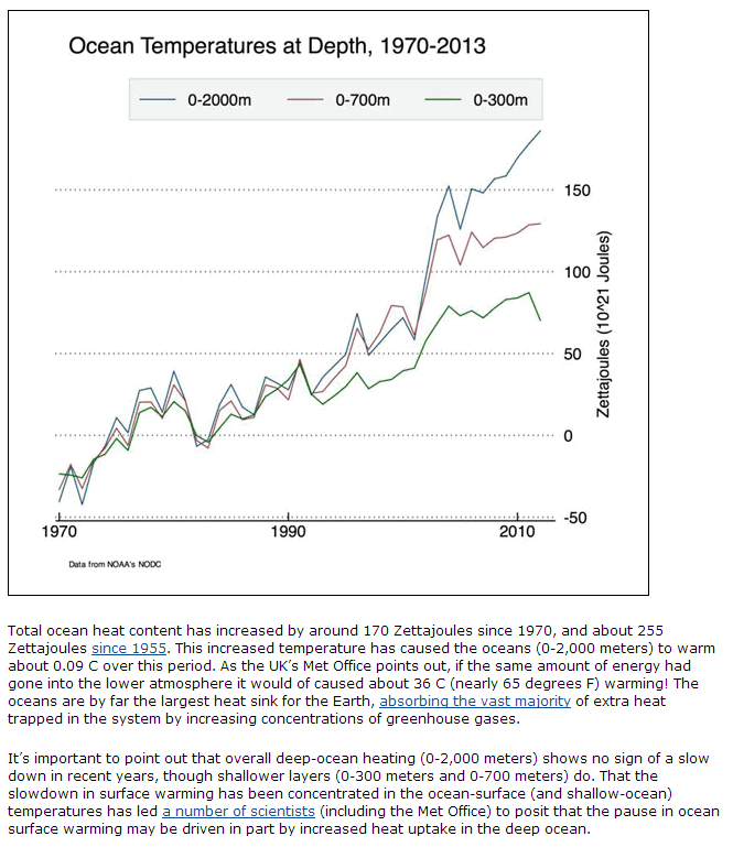
Owing to sampling limitations, it is uncertain whether an increase in the rate of subsurface-ocean heat uptake occurred during the past 15 years (Section 3.2.4). However, it is very likely that the climate system, including the ocean below 700 m depth, has continued to accumulate energy over the period 1998-2010 (Section 3.2.4, Box 3.1). Consistent with this energy accumulation, global mean sea level has continued to rise during 1998-2012, at a rate only slightly and insignificantly lower than during 1993-2012 (Section 3.7). The consistency between observed heat-content and sea level changes yields high confidence in the assessment of continued ocean energy accumulation, which is in turn consistent with the positive radiative imbalance of the climate system (Section 8.5.1; Section 13.3, Box 13.1). By contrast, there is limited evidence that the hiatus in GMST trend has been accompanied by a slower rate of increase in ocean heat content over the depth range 0 to 700 m, when comparing the period 2003-2010 against 1971-2010. There is low agreement on this slowdown, since three of five analyses show a slowdown in the rate of increase while the other two show the increase continuing unabated (Section 3.2.3, Figure 3.2). [Emphasis added by author.]

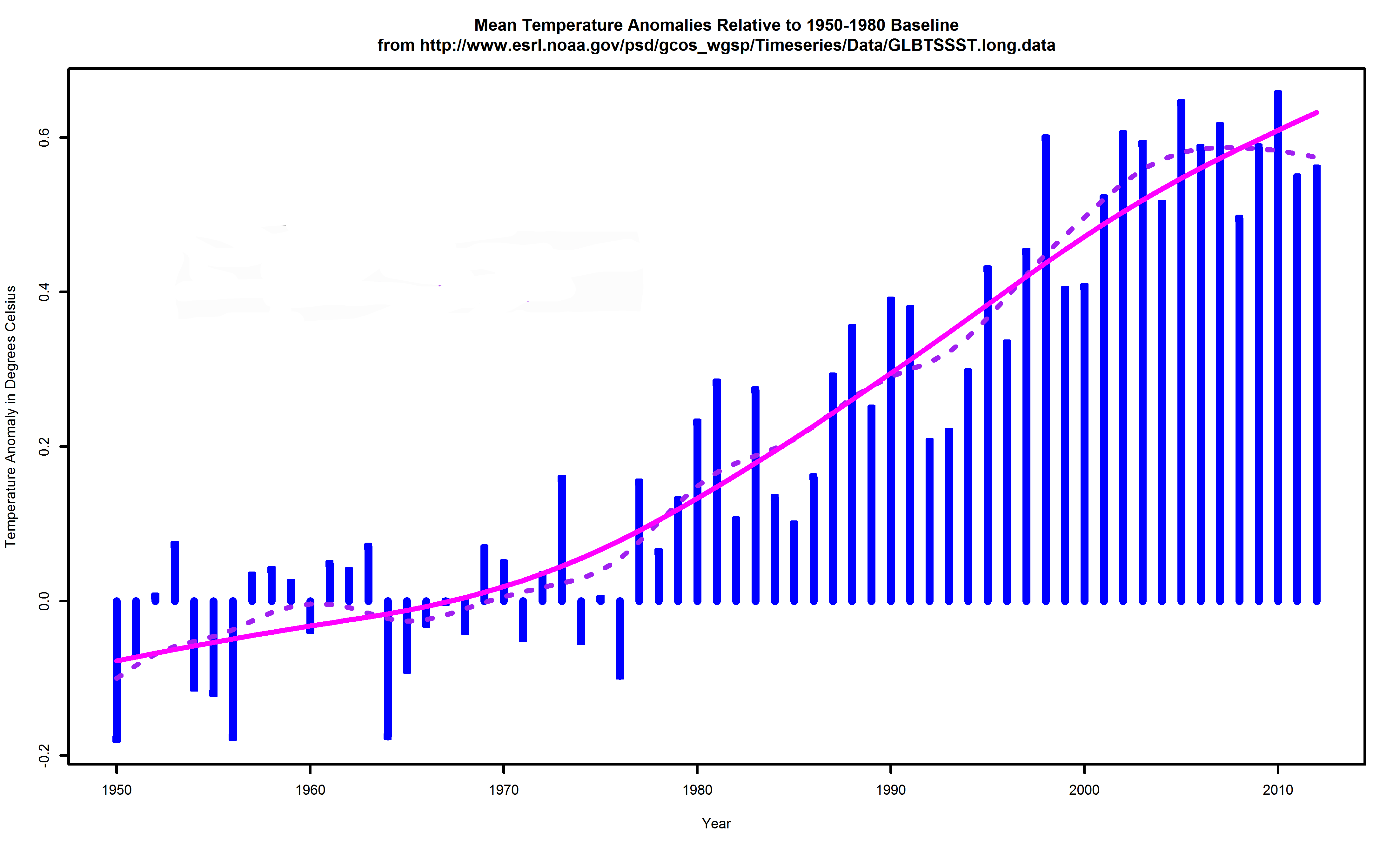
During the 15-year period beginning in 1998, the ensemble of HadCRUT4 GMST trends lies below almost all model-simulated trends (Box 9.2 Figure 1a), whereas during the 15-year period ending in 1998, it lies above 93 out of 114 modelled trends (Box 9.2 Figure 1b; HadCRUT4 ensemble-mean trend $$0.26\,^{\circ}\mathrm{C}$$ per decade, CMIP5 ensemble-mean trend $$0.16\,^{\circ}\mathrm{C}$$ per decade). Over the 62-year period 1951-2012, observed and CMIP5 ensemble-mean trends agree to within $$0.02\,^{\circ}\mathrm{C}$$ per decade (Box 9.2 Figure 1c; CMIP5 ensemble-mean trend $$0.13\,^{\circ}\mathrm{C}$$ per decade). There is hence very high confidence that the CMIP5 models show long-term GMST trends consistent with observations, despite the disagreement over the most recent 15-year period. Due to internal climate variability, in any given 15-year period the observed GMST trend sometimes lies near one end of a model ensemble (Box 9.2, Figure 1a, b; Easterling and Wehner, 2009), an effect that is pronounced in Box 9.2, Figure 1a, because GMST was influenced by a very strong El Ni\~{n}o event in 1998. [Emphasis added by author.]

The contributions of Fyfe, Gillet, and Zwiers ("FGZ") are to (a) pin down this behavior for a 20 year period using the HadCRUT4 data, and, to my mind, more importantly, (b) to develop techniques for evaluating runs of ensembles of climate models like the CMIP5 suite without commissioning specfic runs for the purpose. This, if it were to prove out, would be an important experimental advance, since climate models demand expensive and extensive hardware, and the number of people who know how to program and run them is very limited, possibly a more limiting practical constraint than the hardware.

This is the beginning of a great story, I think, one which both advances an understanding of how our experience of climate is playing out, and how climate science is advancing. FGZ took a perfectly reasonable approach and followed it to its logical conclusion, deriving an inconsistency. There's insight to be won resolving it.

FGZ try to explicitly model trends due to internal variability. They begin with two equations:

$$ M_{ij}(t) &= u^{m}(t) + \text{Eint}_{ij}(t) + \text{Emod}_{i}(t), i = 1, \dots, N^{m}, j= 1, \dots, N_{i} $$
$$ O_{k}(t) &= u^{o}(t) + \text{Eint}^{o}(t) + \text{Esamp}_{k}(t), k = 1, \dots, N^{o} $$

$$i$$ is the model membership index. $$j$$ is the index of the $$i^{\text{th}}$$ model's $$j^{\text{th}}$$ ensemble. $$k$$ runs over bootstrap samples taken from HadCRUT4 observations. Here, $$M_{ij}(t)$$ and $$O_{k}(t)$$ are trends calculated using models or observations, respectively. $$u^{m}(t)$$ and $$u^{o}(t)$$ denote the "true, unknown, deterministic trends due to external forcing" common to models and observations, respectively. $$\text{Eint}_{ij}(t)$$ and $$\text{Eint}^{o}(t)$$ are the perturbations to trends due to internal variability of models and observations. $$\text{Emod}_{i}(t)$$ denotes error in climate model trends for model $$i$$. $$\text{Esamp}_{k}(t)$$ denotes the sampling error in the $$k^{\text{th}}$$ sample. FGZ assume $$\text{Emod}_{i}(t)$$ are exchangeable with each other as well, at least for the same time $$t$$. (See [Di1977, Di1988, Ro2013c, Co2005] for more on exchangeability.) Note that while the internal variability of climate models $$\text{Eint}_{ij}(t)$$ varies from model to model, run to run, and time to time, the 'internal variability of observations', namely $$\text{Eint}^{o}(t)$$, is assumed to only vary with time.

% % The technical innovation FGZ use is to employ bootstrap resampling on the observations ensemble of HadCRUT4 and an ensemble of runs of 38 CMIP5 climate models to perform a two-sample comparison [Ch2008, Da2009, ]. In doing so, they explicitly assume, in the framework above, exchangeability of models. (Later, in the same work, they also make the same calculation assuming exchangeability of models and observations, an innovation too detailed for this present exposition.)

So, what is a bootstrap? In its simplest form, a bootstrap is a nonparametric, often robust, frequentist technique for sampling the distribution of a function of a set of population parameters, generally irrespective of the nature or complexity of that function, or the number of parameters. Since estimates of the variance of that function are themselves functions of population parameters, assuming the variance exists, the bootstrap can also be used to estimate the precision of the first set of samples, where "precision" is the reciprocal of variance. More about the bootstrap is described in an inset.

In the case in question here, with FGZ, the bootstrap is being used to determine if the distribution of surface temperature trends as calculated from observations and the distribution of surface temperature trends as calculated from climate models for the same period have in fact similar means. This is done by examining differences of paired trends, one coming from an observation sample, one coming from a model sample, and assessing the degree of discrepancy based upon the variances of the observations trends distribution and of the models trends distribution.

The equations (6.1) and (6.2) can be re-written:

$$ M_{ij}(t) - \text{Eint}_{ij}(t) = u^{m}(t) + \text{Emod}_{i}(t), i = 1, \dots, N^{m}, j = 1, \dots, N_{i} $$
$$ O_{k}(t) - \text{Eint}^{o}(t) = u^{o}(t) + \text{Esamp}_{k}(t), k = 1, \dots, N^{o} $$

moving the trends in internal variability to the left, calculated side. Both $$\text{Eint}_{ij}(t)$$ and $$\text{Eint}^{o}(t)$$ are not directly observable. Without some additional assumptions, which are not explicitly given in the FGZ paper, such as

$$ \text{Eint}_{ij}(t) \sim \mathcal{N}(0, \Sigma_{\text{model int}}) $$
$$ \text{Eint}^{o}(t) \sim \mathcal{N}(0, \Sigma_{\text{obs int}}) $$

we can't really be sure we're seeing $$O_{k}(t)$$ or $$O_{k}(t) - \text{Eint}^{o}(t)$$, or at least $$O_{k}(t)$$ less the mean of $$\text{Eint}^{o}(t)$$. The same applies to $$M_{ij}(t)$$ and $$\text{Eint}_{ij}(t)$$. Here equations (6.5) and (6.6) describe internal variabilities as being multivariate but zero mean Gaussian random variables. $$\Sigma_{\text{model int}}$$ and $$\Sigma_{\text{obs int}}$$ are covariances among models and among observations. FGZ essentially say these are diagonal with their statement "An implicit assumption is that sampling uncertainty in [observation trends] is independent of uncertainty due to internal variability and also independent of uncertainty in [model trends]". They might not be so, but it is reasonable to suppose their diagonals are strong, and that there is a row-column exchange operator on these covariances which can produce banded matrices.

7. On Reconciliation

The centerpiece of the FGZ result is their Figure 1, reproduced here as Figure 15. Their conclusion, that climate models do not properly capture surface temperature observations for the given periods, is based upon the significant separation of the red density from the grey density, even when measuring that separation using pooled variances. But, surely, a remarkable feature of these graphs is not only the separation of the means of the two densities, but the marked difference in size of the variances of the two densities. Why are climate models so less precise

Figure 15. Figure 1 from Fyfe, Gillet, Zwiers.

than HadCRUT4 observations? Moreover, why do climate models disagree with one another so dramatically? We cannot tell without getting into CMIP5 details, but the same result could be obtained if the climate models came in three Gaussian populations, each with a variance 1.5x that of the observations, but mixed together. We could also obtain the same result if, for some reason, the variance of HadCRUT4 was markedly understated.

That brings us back to the comments about HadCRUT4 made at the end of Section ">3. HadCRUT4 is noted for "drop outs" in observations, where either the quality of an observation on a patch of Earth was poor or the observation was missing altogether for a certain month in history. (To be fair, both GISS and BEST have months where there is no data available, especially in early years of the record.) It also has incomplete coverage [Co2013]. Whether or not values for patches are imputed in some way, perhaps using spatial kriging, or whether or not supports to calculate trends are adjusted to avoid these omissions are decisions in use of these data which are critical to resolving the question [Co2013, Gl2011]. As seen in Section 5, what trends you get depends a lot on how they are done. FGZ did linear trends. These are nice because means of trends have simple relationships with the trends themselves. On the other hand, confining trend estimation to local linear trends binds these estimates to being only supported by pairs of actual samples, however sparse these may be. This has the unfortunate effect of producing a broadly spaced set of trends which, when averaged, appear to be a single, tight distribution, close to the vertical black line of Figure 14, but erasing all the detail available by estimating the density of trends with a robust function of the first time derivative of the series. FGZ might be improved by using such, repairing this drawback and also making it more robust against HadCRUT4's inescapable data drops. As mentioned before, however, we really cannot know, because details of their calculations are not available. (Again, this author suspects this fault lies not with FGZ but a matter of page limits.)

In fact, that was indicated by a recent paper from Cowtan and Way, arguing that the limited coverage of HadCRUT4 might explain the discrepancy Fyfe, Gillet, and Zwiers found. In return Fyfe and Gillet argued that even admitting the corrections for polar regions which Cowtan and Way indicate, the CMIP5 models fall short in accounting for global mean surface temperatures. What could be wrong?

While this has not yet been verified, I suspect there may be a shortcoming in the way which the ensemble of 100 members of HadCRUT4 studies are being used which may explain. In the context of ensemble forecasts depicting future states of the atmosphere, Wilks notes (Section 7.7.1)

Accordingly, the dispersion of a forecast ensemble can at best only approximate the [probability density function] of forecast uncertainty ... In particular, a forecast ensemble may reflect errors both in statistical location (most or all ensemble members being well away from the actual state of the atmosphere, but relatively nearer to each other) and dispersion (either under- or overrepresenting the forecast uncertainty). Often, operational ensemble forecasts are found to exhibit too little dispersion ..., which leads to overconfidence in probability assessment if ensemble relative frequencies are interpreted as estimating probabilities.

In fact, the IPCC reference, Toth, Palmer and others raise the same caution. It could be that the answer to why the variance of the observational data in the Fyfe, Gillet, and Zwiers graph depicted in Figure 15 is so small is that ensemble spread does not properly reflect the true probability density function of the joint distribution of temperatures across Earth. These might be "relatively nearer to each other" than the true dispersion which climate models are accommodating.

If Earth's climate is thought of as a dynamical system, and taking note of the suggestion of Kharin that "There is basically one observational record in climate research", we can do the following thought experiment. Suppose the total state of the Earth's climate system can be captured at one moment in time, no matter how, and the climate can be reinitialized to that state at our whim, again no matter how. What happens if this is done several times, and then the climate is permitted to develop for, say, exactly 100 years on each "run"? What are the resulting states? Also suppose the dynamical "inputs" from the Sun, as a function of time, are held identical during that 100 years, as are dynamical inputs from volcanic forcings, as are human emissions of greenhouse gases. Are the resulting states copies of one another?

No. Stochastic variability in the operation of climate means these end states will be each somewhat different than one another. Then of what use is the "one observation record"? Well, it is arguably better than no observational record. And, in fact, this kind of variability is a major part of the "internal variability" which is often cited in these literature, including by FGZ.

Setting aside the problems of using local linear trends, FGZ's bootstrap approach to the HadCRUT4 ensemble is an attempt to imitate these various runs of Earth's climate. The trouble is, the frequentist bootstrap can only replicate values of observations actually seen. (See inset.) In this case, these replications are those of the HadCRUT4 ensembles. It will never produce values in-between and, as the parameters of temperature anomalies are in general continuous measures, allowing for in-between values seems a reasonable thing to do.

No algorithm can account for a dispersion which is not reflected in the variability of the ensemble. If the dispersion of HadCRUT4 is too small, it could be corrected using ensemble MOS methods (Section 7.7.1.) In any case, underdispersion could explain the remarkable difference in variances of populations seen in Figure 15. I think there's yet another way.

Consider equations (6.1) and (6.2) again. Recall, here, $$i$$ denotes the $$i^{\text{th}}$$ model and $$j$$ denotes the $$j^{\text{th}}$$ run of model $$i$$. Instead of $$k$$, however, a bootstrap resampling of the HadCRUT4 ensembles, let $$\mathpzc{l}$$ run over all the 100 ensemble members provided, let $$\mathpzc{j}$$ run over the 2592 patches on Earth's surface, and let $$\kappa$$ run over the 1967 monthly time steps. Reformulate equations (6.1) and (6.2), instead, as

$$ M_{\kappa} = u_{\kappa} + \sum_{i = 1}^{N^{m}} x_{i} \left(\text{Emod}_{i\kappa} + \text{Eint}_{i\kappa}\right) $$
$$ O_{\kappa} = u_{\kappa} + x_{0} \text{Eint}^{\mathbf{o}}_{\kappa} + \sum_{\mathpzc{j} = 1}^{2592} x_{\mathpzc{j}} \text{Esamp}_{\mathpzc{j}\kappa} $$

Now, $$u_{\kappa}$$ is a common trend at time tick $$\kappa$$ and $$\text{Emod}_{i\kappa}$$ and $$\text{Eint}_{i\kappa}$$ are deflections from from that trend due to modeling error and internal variability in the $$i^{\text{th}}$$ model, respectively, at time tick $$\kappa$$. Similarly, $$\text{Eint}^{\mathbf{o}}_{\kappa}$$ denotes deflections from the common trend baseline $$u$$ due to internal variability as seen by the HadCRUT4 observational data at time tick $$\kappa$$, and $$\text{Esamp}_{\mathpzc{j}\kappa}$$ denotes the deflection from the common baseline due to sampling error in the $$\mathpzc{j}^{\text{th}}$$ patch at time tick $$\kappa$$. $$x_{\iota}$$ are indicator variables. This is the setup for an analysis of variance or ANOVA, preferably a Bayesian one (Sections 14.1.6, 18.1). In equation (7.1), successive model runs $$j$$ for model $$i$$ are used to estimate $$\text{Emod}_{i\kappa}$$ and $$\text{Eint}_{i\kappa}$$ for every $$\kappa$$. In equation (7.2), different ensemble members $$\mathpzc{l}$$ are used to estimate $$\text{Eint}^{\mathbf{o}}_{\kappa}$$ and $$\text{Esamp}_{\mathpzc{j}\kappa}$$ for every $$\kappa$$. Coupling the two gives a common estimate of $$u_{\kappa}$$. There's considerable flexibility in how model runs or ensemble members are used for this purpose, opportunities for additional differentiation and ability to incorporate information about relationships among models or among observations. For instance, models might be described relative to a Bayesian model average [Ra2005]. Observations might be described relative to a common or slowly varying spatial trend, reflecting dependencies among $$\mathpzc{j}$$ patches. Here, differences between observations and models get explicitly allocated to modeling error and internal variability for models, and sampling error and internal variability for observations.

More work needs to be done to assess the proper virtues of the FGZ technique, even without modification. A device like that Rohde used to compare BEST temperature observations with HadCRUT4 and GISS, one of supplying the FGZ procedure with synthetic data, would be perhaps the most informative regarding its character. Alternatively, if an ensemble MOS method were devised and applied to HadCRUT4, it might better reflect a true spread of possibilities. Because a dataset like HadCRUT4 records just one of many possible observational records the Earth might have exhibited, it would be useful to have a means of elaborating what those other possibilities were, given the single observational trace.

Regarding climate models, while they will inevitably disagree from a properly elaborated set of observations in the particulars of their statistics, in my opinion, the goal should be to strive to match the distributions of solutions these two instruments of study on their first few moments by improving both. While, statistical equivalence is all that's sought, we're not there yet. Assessing parametric uncertainty of observations hand-in-hand with the model builders seems to be a sensible route. Indeed, this is important. In review of the Cowtan and Way result, one based upon kriging, Kintisch summarizes the situation as reproduced in Table 1, a reproduction of his table on page 348 of the reference [Co2013, Gl2011, Ki2014]:

Table 1. **Getting warmer.** New method brings measured temperatures closer to projections. Added in quotation: "Climate models" refers to the CMIP5 series. "NASA data set" is GISS. "HadCRUT data set" is HadCRUT4. "Cowtan/Way" is from their paper. **Note values are per decade, not per year.**
TEMPERATURE TRENDS
1997-2012
Source	Warming ($$^{\circ}\,\mathrm{C}$$/decade)
Climate models	0.102-0.412
NASA data set	0.080
HadCRUT data set	0.046
Cowtan/Way	0.119

Note that these estimates of trends, once divided by 10 years/decade to convert to a per year change in temperature, all fall well within the slope estimates depicted in the summary Figure 14. Note, too, how low the HadCRUT trend is.

If the FGZ technique, or any other, can contribute to this elucidation, it is most welcome.

As an example Lee reports how the GLOMAP model of aerosols was systematically improved using such careful statistical consideration. It seems likely to be a more rewarding way than "black box" treatments. Incidently, Dr Lindsay Lee's article was runner-up in the Significance/Young Statisticians Section writers' competition. It's great to see bright young minds charging in to solve these problems!

The bootstrap is a general name for a resampling technique, most commonly associated with what is more properly called the frequentist bootstrap. Given a sample of observations, $$\mathring{Y} = \{y_{1}, y_{2}, \dots, y_{n}\}$$, the bootstrap principle says that in a wide class of statistics and for certain minimum sizes of $$n$$, the sampling density of a statistic $$h(Y)$$ from a population of all $$Y$$, where $$\mathring{Y}$$ is a single observation, can be approximated by the following procedure. Sample $$\mathring{Y}$$ $$M$$ times with replacement to obtain $$M$$ samples each of size $$n$$ called $$\tilde{Y}_{k}$$, $$k = 1, \dots, M$$. For each $$\tilde{Y}_{k}$$, calculate $$h(\tilde{Y}_{k})$$ so as to obtain $$H = h_{1}, h_{2}, \dots, h_{M}$$. The set $$H$$ so obtained is an approximation of the sampling density of $$h(Y)$$ from a population of all $$Y$$. Note that because $$\mathring{Y}$$ is sampled, only elements of that original set of observations will ever show up in any $$\tilde{Y}_{k}$$. This is true even if $$Y$$ is drawn from an interval of the real numbers. This is where a Bayesian bootstrap might be more suitable.

In a Bayesian bootstrap, the set of possibilities to be sampled are specified using a prior distribution on $$Y$$ [Da2009, Section 10.5]. A specific observation of $$Y$$, like $$\mathring{Y}$$, is use to update the probability density on $$Y$$, and then values from $$Y$$ are drawn in proportion to this updated probability. Thus, values in $$Y$$ never in $$\mathring{Y}$$ might be drawn. Both bootstraps will, under similar conditions, preserve the sampling distribution of $$Y$$.

8. Summary

Various geophysical datasets recording global surface temperature anomalies suggest a slowdown in anomalous global warming from historical baselines. Warming is increasing, but not as fast, and much of the media attention to this is reacting to the second time derivative of temperature, which is negative, not the first time derivative, its rate of increase. Explanations vary. In one important respect, 20 or 30 years is an insufficiently long time to assess the state of the climate system. In another, while the global surface temperature increase is slowing, oceanic temperatures continue to soar, at many depths. Warming might even decrease. None of these seem to pose a challenge to the geophysics of climate, which has substantial support both from experimental science and ab initio calculations. An interesting discrepancy is noted by Fyfe, Gillet, and Zwiers, although their calculation could be improved both by using a more robust estimator for trends, and by trying to integrate out anomalous temperatures due to internal variability in their models, because much of it is not separately observable. Nevertheless, Fyfe, Gillet, and Zwiers may have done the field a great service, making explicit a discrepancy which enables students of datasets like the important HadCRUT4 to discover an important limitation, that their dispersion across ensembles does not properly reflect the set of Earth futures which one might wish they did and, in their failure for users who think of the ensemble as representing such futures, give them a dispersion which is significantly smaller than what we might know.

The Azimuth Project can contribute, and I am planning subprojects to pursue my suggestions in Section 7, those of examining HadCRUT4 improvements using MOS ensembles, a Bayesian bootstrap, or the Bayesian ANOVA described there. Beyond trends in mean surface temperatures, there's another more challenging statistical problem involving trends in sea levels which awaits investigation [Le2012b, Hu2010].

Working out these kinds of details is the process of science at its best, and many disciplines, not least mathematics, statistics, and signal processing, have much to contribute to the methods and interpretations of these series data. It is possible too much is being asked of a limited data set, and we have not yet observed enough of climate system response to tell anything definitive. But the urgency to act responsibly given scientific predictions remains.

Bibliography

CREDENTIALS: I have taken courses in geology from Binghamton University, but the rest of my knowledge of climate science is from reading the technical literature, principally publications from the American Geophysical Union and the American Meteorological Society, and self-teaching, from textbooks like Pierrehumbert. I seek to find ways where my different perspective on things canhelp advance and explain the climate science enterprise. I also apply my skills to working local environmental problems, ranging from inferring people's use of energy in local municipalities, as well as studying things like trends in solid waste production at the same scales using Bayesian inversions. I am fortunate that techniques used in my professional work and those in these problems overlap so much. I am a member of the American Statistical Association, the American Geophysical Union, theAmerican Meteorological Association, the International Society for Bayesian Analysis, as well as the IEEE and its signal processing society.
Yo2014: D. S. Young, "Bond. James Bond. A statistical look at cinema�s most famous spy", CHANCE Magazine, 27(2), 2014, 21-27, http://chance.amstat.org/2014/04/james-bond/.
Ca2014a: S. Carson, Science of Doom, a Web site devoted to atmospheric radiation physics and forcings, last accessed 7^th February 2014.
Pi2012: R. T. Pierrehumbert, Principles of Planetary Climate, Cambridge University Press, 2010, reprinted 2012.
Pi2011: R. T. Pierrehumbert, "Infrared radiative and planetary temperature", Physics Today, January 2011, 33-38.
Pe2006: G. W. Petty, A First Course in Atmospheric Radiation, 2^nd edition, Sundog Publishing, 2006.
Le2012a: S. Levitus, J. I. Antonov, T. P. Boyer, O. K. Baranova, H. E. Garcia, R. A. Locarnini, A. V. Mishonov, J. R. Reagan, D. Seidov, E. S. Yarosh, and M. M. Zweng, "World ocean heat content and thermosteric sea level change (0-2000 m), 1955-2010", Geophysical Research Letters, 39, L10603, 2012, http://dx.doi.org/10.1029/2012GL051106.
Le2012b: S. Levitus, J. I. Antonov, T. P. Boyer, O. K. Baranova, H. E. Garcia, R. A. Locarnini, A. V. Mishonov, J. R. Reagan, D. Seidov, E. S. Yarosh, and M. M. Zweng, "World ocean heat content and thermosteric sea level change (0-2000 m), 1955-2010: supplementary information", Geophysical Research Letters, 39, L10603, 2012, http://onlinelibrary.wiley.com/doi/10.1029/2012GL051106/suppinfo.
Sm2009: R. L. Smith, C. Tebaldi, D. Nychka, L. O. Mearns, "Bayesian modeling of uncertainty in ensembles of climate models", Journal of the American Statistical Association, 104(485), March 2009.
NOMENCLAT: The nomenclature can be confusing. With respect to observations, variability arising due to choice of method is sometimes called structural uncertainty [Mo2012, Th2005].
Kr2014: J. P. Krasting, J. P. Dunne, E. Shevliakova, R. J. Stouffer (2014), "Trajectory sensitivity of the transient climate response to cumulative carbon emissions", Geophysical Research Letters, 41, 2014, http://dx.doi.org/10.1002/2013GL059141.
Sh2014a: D. T. Shindell, "Inhomogeneous forcing and transient climate sensitivity", Nature Climate Change, 4, 2014, 274-277, http://dx.doi.org/10.1038/nclimate2136.
Sh2014b: D. T. Shindell, "Shindell: On constraining the Transient Climate Response", RealClimate, http://www.realclimate.org/index.php?p=17134, 8^th April 2014.
Sa2011: B. M. Sanderson, B. C. O�Neill, J. T. Kiehl, G. A. Meehl, R. Knutti, W. M. Washington, "The response of the climate system to very high greenhouse gas emission scenarios", Environmental Research Letters, 6, 2011, 034005, http://dx.doi.org/10.1088/1748-9326/6/3/034005.
Em2011: K. Emanuel, "Global warming effects on U.S. hurricane damage", Weather, Climate, and Society, 3, 2011, 261-268, http://dx.doi.org/10.1175/WCAS-D-11-00007.1.
Sm2011: L. A. Smith, N. Stern, "Uncertainty in science and its role in climate policy", Philosophical Transactions of the Royal Society A, 269, 2011 369, 1-24, http://dx.doi.org/10.1098/rsta.2011.0149.
Le2010: M. C. Lemos, R. B. Rood, "Climate projections and their impact on policy and practice", WIREs Climate Change, 1, September/October 2010, http://dx.doi.org/10.1002/wcc.71.
Sc2014: G. A. Schmidt, D. T. Shindell, K. Tsigaridis, "Reconciling warming trends", Nature Geoscience, 7, 2014, 158-160, http://dx.doi.org/10.1038/ngeo2105.
Be2013: "Examining the recent "pause" in global warming", Berkeley Earth Memo, 2013, http://static.berkeleyearth.org/memos/examining-the-pause.pdf.
Mu2013a: R. A. Muller, J. Curry, D. Groom, R. Jacobsen, S. Perlmutter, R. Rohde, A. Rosenfeld, C. Wickham, J. Wurtele, "Decadal variations in the global atmospheric land temperatures", Journal of Geophysical Research: Atmospheres, 118(11), 2013, 5280-5286, http://dx.doi.org/10.1002/jgrd.50458.
Mu2013b: R. Muller, "Has global warming stopped?", Berkeley Earth Memo, September 2013, http://static.berkeleyearth.org/memos/has-global-warming-stopped.pdf.
Br2006: P. Brohan, J. Kennedy, I. Harris, S. Tett, P. D. Jones, "Uncertainty estimates in regional and global observed temperature changes: A new data set from 1850", Journal of Geophysical Research \textendash Atmospheres, 111(D12), 27 June 2006, http://dx.doi.org/10.1029/2005JD006548.
Co2013: K. Cowtan, R. G. Way, "Coverage bias in the HadCRUT4 temperature series and its impact on recent temperature trends", Quarterly Journal of the Royal Meteorological Society, 2013, http://dx.doi.org/10.1002/qj.2297.
Fy2013: J. C. Fyfe, N. P. Gillett, F. W. Zwiers, "Overestimated global warming over the past 20 years", Nature Climate Change, 3, September 2013, 767-769, and online at http://dx.doi.org/10.1038/nclimate1972.
Ha2013: E. Hawkins, "Comparing global temperature observations and simulations, again", Climate Lab Book, http://www.climate-lab-book.ac.uk/2013/comparing-observations-and-simulations-again/, 28^th May 2013.
Ha2014: A. Hannart, A. Ribes, P. Naveau, "Optimal fingerprinting under multiple sources of uncertainty", Geophysical Research Letters, 41, 2014, 1261-1268, http://dx.doi.org/10.1002/2013GL058653.
Ka2013a: R. W. Katz, P. F. Craigmile, P. Guttorp, M. Haran, Bruno Sans'{o}, M.L. Stein, "Uncertainty analysis in climate change assessments", Nature Climate Change, 3, September 2013, 769-771 ("Commentary").
Sl2013: J. Slingo, "Statistical models and the global temperature record", Met Office, May 2013, http://www.metoffice.gov.uk/media/pdf/2/3/Statistical_Models_Climate_Change_May_2013.pdf.
Tr2013: K. Trenberth, J. Fasullo, "An apparent hiatus in global warming?", Earth�s Future, 2013, http://dx.doi.org/10.1002/2013EF000165.
Mo2012: C. P. Morice, J. J. Kennedy, N. A. Rayner, P. D. Jones, "Quantifying uncertainties in global and regional temperature change using an ensemble of observational estimates: The HadCRUT4 data set", Journal of Geophysical Research, 117, 2012, http://dx.doi.org/10.1029/2011JD017187. See also http://www.metoffice.gov.uk/hadobs/hadcrut4/data/current/download.html where the 100 ensembles can be found.
Sa2012: B. D. Santer, J. F. Painter, C. A. Mears, C. Doutriaux, P. Caldwell, J. M. Arblaster, P. J. Cameron-Smith, N. P. Gillett, P. J. Gleckler, J. Lanzante, J. Perlwitz, S. Solomon, P. A. Stott, K. E. Taylor, L. Terray, P. W. Thorne, M. F. Wehner, F. J. Wentz, T. M. L. Wigley, L. J. Wilcox, C.-Z. Zou, "Identifying human infuences on atmospheric temperature", Proceedings of the National Academy of Sciences, (PNAS), 29^th November 2012, http://dx.doi.org/10.1073/pnas.1210514109.
Ke2011a: J. J. Kennedy, N. A. Rayner, R. O. Smith, D. E. Parker, M. Saunby, "Reassessing biases and other uncertainties in sea-surface temperature observations measured in situ since 1850, part 1: measurement and sampling uncertainties", Journal of Geophysical Research: Atmospheres (1984-2012), 116(D14), 27 July 2011, http://dx.doi.org/10.1029/2010JD015218. \begin{changebar}
Kh2008a: S. Kharin, "Statistical concepts in climate research: Some misuses of statistics in climatology", Banff Summer School, 2008, part 1 of 3. Slide 7, "Climatology is a one-experiment science. There is basically one observational record in climate", http://www.atmosp.physics.utoronto.ca/C-SPARC/ss08/lectures/Kharin-lecture1.pdf.
Kh2008b: S. Kharin, "Climate Change Detection and Attribution: Bayesian view", Banff Summer School, 2008, part 3 of 3, http://www.atmosp.physics.utoronto.ca/C-SPARC/ss08/lectures/Kharin-lecture3.pdf. \end{changebar}
Le2005: T. C. K. Lee, F. W. Zwiers, G. C. Hegerl, X. Zhang, M. Tsao, "A Bayesian climate change detection and attribution assessment", Journal of Climate, 18, 2005, 2429-2440.
De1982: M. H. DeGroot, S. Fienberg, "The comparison and evaluation of forecasters", The Statistician, 32(1-2), 1983, 12-22.
Ro2013a: R. Rhode, R. A. Muller, R. Jacobsen, E. Muller, S. Perlmutter, A. Rosenfeld, J. Wurtele, D. Groom, C. Wickham, "A new estimate of the average Earth surface land temperature spanning 1753 to 2011", Geoinformatics & Geostatistics: An Overview, 1(1), 2013, http://dx.doi.org/10.4172/2327-4581.1000101.
Ke2011b: J. J. Kennedy, N. A. Rayner, R. O. Smith, D. E. Parker, M. Saunby, "Reassessing biases and other uncertainties in sea-surface temperature observations measured in situ since 1850, part 2: Biases and homogenization", Journal of Geophysical Research: Atmospheres (1984-2012), 116(D14), 27 July 2011, http://dx.doi.org/10.1029/2010JD015220.
Ro2013b: R. Rohde, "Comparison of Berkeley Earth, NASA GISS, and Hadley CRU averaging techniques on ideal synthetic data", Berkeley Earth Memo, January 2013, http://static.berkeleyearth.org/memos/robert-rohde-memo.pdf.
En2014: M. H. England, S. McGregor, P. Spence, G. A. Meehl, A. Timmermann, W. Cai, A. S. Gupta, M. J. McPhaden, A. Purich, A. Santoso, "Recent intensification of wind-driven circulation in the Pacific and the ongoing warming hiatus", Nature Climate Change, 4, 2014, 222-227, http://dx.doi.org/10.1038/nclimate2106. See also http://www.realclimate.org/index.php/archives/2014/02/going-with-the-wind/.
Fy2014: J. C. Fyfe, N. P. Gillett, "Recent observed and simulated warming", Nature Climate Change, 4, March 2014, 150-151, http://dx.doi.org/10.1038/nclimate2111.
Ta2013: "Tamino", "el Ni\~{n}o and the Non-Spherical Cow", Open Mind blog, http://tamino.wordpress.com/2013/09/02/el-nino-and-the-non-spherical-cow/, 2^nd September 2013.
Fy2013s: Supplement to J. C. Fyfe, N. P. Gillett, F. W. Zwiers, "Overestimated global warming over the past 20 years", Nature Climate Change, 3, September 2013, online at http://www.nature.com/nclimate/journal/v3/n9/extref/nclimate1972-s1.pdf.
IONIZING: There are tiny amounts of heating due to impinging ionizing radiation from space, and changes in Earth's magnetic field.
Ki1997: J. T. Kiehl, K. E. Trenberth, "Earth's annual global mean energy budget", Bulletin of the American Meteorological Society, 78(2), 1997, http://dx.doi.org/10.1175/1520-0477(1997)078<0197:EAGMEB>2.0.CO;2.
Tr2009: K. Trenberth, J. Fasullo, J. T. Kiehl, "Earth's global energy budget", Bulletin of the American Meteorological Society, 90, 2009, 311�323, http://dx.doi.org/10.1175/2008BAMS2634.1.
IP2013: IPCC, 2013: Climate Change 2013: The Physical Science Basis. Contribution of Working Group I to the Fifth Assessment Report of the Intergovernmental Panel on Climate Change [Stocker, T.F., D. Qin, G.-K. Plattner, M. Tignor, S.K. Allen, J. Boschung, A. Nauels, Y. Xia, V. Bex and P.M. Midgley (eds.)]. Cambridge University Press, Cambridge, United Kingdom and New York, NY, USA, 1535 pp.
Ve2012: A. Vehtari, J. Ojanen, "A survey of Bayesian predictive methods for model assessment, selection and comparison", Statistics Surveys, 6 (2012), 142-228, http://dx.doi.org/10.1214/12-SS102.
Ge1998: J. Geweke, "Simulation Methods for Model Criticism and Robustness Analysis", in Bayesian Statistics 6, J. M. Bernardo, J. O. Berger, A. P. Dawid and A. F. M. Smith (eds.), Oxford University Press, 1998.
Co2006: P. Congdon, Bayesian Statistical Modelling, 2^nd edition, John Wiley & Sons, 2006.
Fe2011b: D. Ferreira, J. Marshall, B. Rose, "Climate determinism revisited: Multiple equilibria in a complex climate model", Journal of Climate, 24, 2011, 992-1012, http://dx.doi.org/10.1175/2010JCLI3580.1.
Bu2002: K. P. Burnham, D. R. Anderson, Model Selection and Multimodel Inference, 2^nd edition, Springer-Verlag, 2002.
Ea2014a: S. Easterbrook, "What Does the New IPCC Report Say About Climate Change? (Part 4): Most of the heat is going into the oceans", 11^th April 2014, at the Azimuth blog, http://johncarlosbaez.wordpress.com/2014/04/11/what-does-the-new-ipcc-report-say-about-climate-change-part-4/.
Ko2014: Y. Kostov, K. C. Armour, and J. Marshall, "Impact of the Atlantic meridional overturning circulation on ocean heat storage and transient climate change", Geophysical Research Letters, 41, 2014, 2108�2116, http://dx.doi.org/10.1002/2013GL058998.
Me2011: G. A. Meehl, J. M. Arblaster, J. T. Fasullo, A. Hu.K. E. Trenberth, "Model-based evidence of deep-ocean heat uptake during surface-temperature hiatus periods", Nature Climate Change, 1, 2011, 360�364, http://dx.doi.org/10.1038/nclimate1229.
Me2013: G. A. Meehl, A. Hu, J. M. Arblaster, J. Fasullo, K. E. Trenberth, "Externally forced and internally generated decadal climate variability associated with the Interdecadal Pacific Oscillation", Journal of Climate, 26, 2013, 7298�7310, http://dx.doi.org/10.1175/JCLI-D-12-00548.1.
Ha2010: J. Hansen, R. Ruedy, M. Sato, and K. Lo, "Global surface temperature change", Reviews of Geophysics, 48(RG4004), 2010, http://dx.doi.org/10.1029/2010RG000345.
GISS-BEST: 3.667 (GISS) versus 3.670 (BEST).
SPAR: The smoothing parameter is a constant which weights a penalty term proportional to the second directional derivative of the curve. The effect is that if a candidate spline is chosen which is very bumpy, this candidate is penalized and will only be chosen if the data demands it. There is more said about choice of such parameters in the caption of Figure reference.
Ea2009: D. R. Easterling, M. F. Wehner, "Is the climate warming or cooling?", Geophysical Research Letters, 36, L08706, 2009, http://dx.doi.org/10.1029/2009GL037810.
HIATUS: The term hiatus has a formal meaning in climate science, as described by the IPCC itself (Box TS.3).
Ea2000: D. J. Easterbrook, D. J. Kovanen, "Cyclical oscillation of Mt. Baker glaciers in response to climatic changes and their correlation with periodic oceanographic changes in the northeast Pacific Ocean", 32, 2000, Proceedings of the Geological Society of America, Abstracts with Program, page 17, http://myweb.wwu.edu/dbunny/pdfs/dje_abstracts.pdf, abstract reviewed 23^rd April 2014.
Ea2001: D. J. Easterbrook, "The next 25 years: global warming or global cooling? Geologic and oceanographic evidence for cyclical climatic oscillations", 33, 2001, Proceedings of the Geological Society of America, Abstracts with Program, page 253, http://myweb.wwu.edu/dbunny/pdfs/dje_abstracts.pdf, abstract reviewed 23^rd April 2014.
Ea2005: D. J. Easterbrook, "Causes and effects of abrupt, global, climate changes and global warming", Proceedings of the Geological Society of America, 37, 2005, Abstracts with Program, page 41, http://myweb.wwu.edu/dbunny/pdfs/dje_abstracts.pdf, abstract reviewed 23^rd April 2014.
Ea2006a: D. J. Easterbrook, "The cause of global warming and predictions for the coming century", Proceedings of the Geological Society of America, 38(7), Astracts with Programs, page 235, http://myweb.wwu.edu/dbunny/pdfs/dje_abstracts.pdf, abstract reviewed 23^rd April 2014.
Ea2006b: D. J. Easterbrook, 2006b, "Causes of abrupt global climate changes and global warming predictions for the coming century", Proceedings of the Geological Society of America, 38, 2006, Abstracts with Program, page 77, http://myweb.wwu.edu/dbunny/pdfs/dje_abstracts.pdf, abstract reviewed 23^rd April 2014.
Ea2007: D. J. Easterbrook, "Geologic evidence of recurring climate cycles and their implications for the cause of global warming and climate changes in the coming century", Proceedings of the Geological Society of America, 39(6), Abstracts with Programs, page 507, http://myweb.wwu.edu/dbunny/pdfs/dje_abstracts.pdf, abstract reviewed 23^rd April 2014.
Ea2008: D. J. Easterbrook, "Correlation of climatic and solar variations over the past 500 years and predicting global climate changes from recurring climate cycles", Proceedings of the International Geological Congress, 2008, Oslo, Norway.
Wi2007: J. K. Willis, J. M. Lyman, G. C. Johnson, J. Gilson, "Correction to 'Recent Cooling of the Upper Ocean"', Geophysical Research Letters, 34, L16601, 2007, http://dx.doi.org/10.1029/2007GL030323.
Ra2006: N. Rayner, P. Brohan, D. Parker, C. Folland, J. Kennedy, M. Vanicek, T. Ansell, S. Tett, "Improved Analyses of Changes and Uncertainties in Sea Surface Temperature Measured In Situ since the Mid-Nineteenth Century: The HadSST2 Dataset", Journal of Climate, 19, 1 February 2006, http://dx.doi.org/10.1175/JCLI3637.1.
Pi2006: R. Pielke, Sr, "The Lyman et al Paper 'Recent Cooling In the Upper Ocean' Has Been Published", blog entry, September 29, 2006, 8:09 AM, https://pielkeclimatesci.wordpress.com/2006/09/29/the-lyman-et-al-paper-recent-cooling-in-the-upper-ocean-has-been-published/, last accessed 24^th April 2014.
Ko2013: Y. Kosaka, S.-P. Xie, "Recent global-warming hiatus tied to equatorial Pacific surface cooling", Nature, 501, 2013, 403�407, http://dx.doi.org/10.1038/nature12534.
Ke1998: C. D. Keeling, "Rewards and penalties of monitoring the Earth", Annual Review of Energy and the Environment, 23, 1998, 25�82, http://dx.doi.org/10.1146/annurev.energy.23.1.25.
Wa1990: G. Wahba, Spline Models for Observational Data, Society for Industrial and Applied Mathematics (SIAM), 1990.
Go1979: G. H. Golub, M. Heath, G. Wahba, "Generalized cross-validation as a method for choosing a good ridge parameter", Technometrics, 21(2), May 1979, 215-223, http://www.stat.wisc.edu/~wahba/ftp1/oldie/golub.heath.wahba.pdf.
Cr1979: P. Craven, G. Wahba, "Smoothing noisy data with spline functions: Estimating the correct degree of smoothing by the method of generalized cross-validation", Numerische Mathematik, 31, 1979, 377-403, http://www.stat.wisc.edu/~wahba/ftp1/oldie/craven.wah.pdf.
Sa2013: S. Särkkä, Bayesian Filtering and Smoothing, Cambridge University Press, 2013.
Co2009: P. S. P. Cowpertwait, A. V. Metcalfe, Introductory Time Series With R, Springer, 2009.
Ko2005: R. Koenker, Quantile Regression, Cambridge University Press, 2005.
Du2012: J. Durbin, S. J. Koopman, Time Series Analysis by State Space Methods, Oxford University Press, 2012.
PROCESS-VARIANCE: Here, the process variance was taken here to be $$\frac{1}{50}$$ of the observations variance.
PROBABILITIES: "In this Report, the following terms have been used to indicate the assessed likelihood of an outcome or a result: Virtually certain $$99-100$$\% probability, Very likely$$90-100$$\%, Likely $$66-100$$\%, About as likely as not $$33-66$$\%, Unlikely 0-33\%, Very unlikely 0-10\%, Exceptionally unlikely 0-1\%. Additional terms (Extremely likely:$$95-100$$\%, More likely than not $$>50-100$$\%, and Extremely unlikely 0-5\%) may also be used when appropriate. Assessed likelihood is typeset in italics, e.g., verylikely (see Section 1.4 and Box TS.1 for more details)."
Ki2013: E. Kintsch, "Researchers wary as DOE bids to build sixth U.S. climate model", Science, 341(6151), 13^th September 2013, page 1160, http://dx.doi.org/10.1126/science.341.6151.1160.
IFUNG: ""It's great there's a new initiative," says modeler Inez Fung of DOE's Lawrence Berkeley National Laboratory and the University of California, Berkeley. "But all the modeling efforts are very short-handed. More brains working on one set of code would be better than working separately"".
EXCHANGE: Exchangeability is a weaker assumption than independence. Random variables are exchangeable if their joint distribution only depends upon the set of variables, and not their order [Di1977, Di1988, Ro2013c]. Note the caution in Coolen.
Di1977: P. Diaconis, "Finite forms of de Finetti's theorem on exchangeability", Synthese, 36, 1977, 271-281.
Di1988: P. Diaconis, "Recent progress on de Finetti's notions of exchangeability", Bayesian Statistics, 3, 1988, 111-125.
Ro2013c: J.C. Rougier, M. Goldstein, L. House, "Second-order exchangeability analysis for multi-model ensembles", Journal of the American Statistical Association, 108, 2013, 852-863, http://dx.doi.org/10.1080/01621459.2013.802963.
Co2005: F. P. A. Coolen, "On nonparametric predictive inference and objective Bayesianism", Journal of Logic, Language and Information, 15, 2006, 21-47, http://dx.doi.org/10.1007/s10849-005-9005-7. ("Generally, though, both for frequentist and Bayesian approaches, statisticians are often happy to assume exchangeability at the prior stage. Once data are used in combination with model assumptions, exchangeability no longer holds �post-data� due to the influence of modelling assumptions, which effectively are based on mostly subjective input added to the information from the data.").
Ch2008: M. R. Chernick, Bootstrap Methods: A Guide for Practitioners and Researches, 2^nd edition, 2008, John Wiley & Sons.
Da2009: A. C. Davison, D. V. Hinkley, Bootstrap Methods and their Application, first published 1997, 11^th printing, 2009, Cambridge University Press.
Mu2007: M. Mudelsee, M. Alkio, "Quantifying effects in two-sample environmental experiments using bootstrap condidence intervals", Environmental Modelling and Software, 22, 2007, 84-96, http://dx.doi.org/10.1016/j.envsoft.2005.12.001.
Wi2011: D. S. Wilks, Statistical Methods in the Atmospheric Sciences, 3^rd edition, 2011, Academic Press.
Pa2006: T. N. Palmer, R. Buizza, R. Hagedon, A. Lawrence, M. Leutbecher, L. Smith, "Ensemble prediction: A pedagogical perspective", ECMWF Newsletter, 106, 2006, 10�17.
To2001: Z. Toth, Y. Zhu, T. Marchok, "The use of ensembles to identify forecasts with small and large uncertainty", Weather and Forecasting, 16, 2001, 463�477, http://dx.doi.org/10.1175/1520-0434(2001)016<0463:TUOETI>2.0.CO;2.
Le2013a: L. A. Lee, K. J. Pringle, C. I. Reddington, G. W. Mann, P. Stier, D. V. Spracklen, J. R. Pierce, K. S. Carslaw, "The magnitude and causes of uncertainty in global model simulations of cloud condensation nuclei", Atmospheric Chemistry and Physics Discussion, 13, 2013, 6295-6378, http://www.atmos-chem-phys.net/13/9375/2013/acp-13-9375-2013.pdf.
Gl2011: D. M. Glover, W. J. Jenkins, S. C. Doney, Modeling Methods for Marine Science, Cambridge University Press, 2011.
Ki2014: E. Kintisch, "Climate outsider finds missing global warming", Science, 344(6182), 25^th April 2014, page 348, http://dx.doi.org/10.1126/science.344.6182.348.
GL2011: D. M. Glover, W. J. Jenkins, S. C. Doney, Modeling Methods for Marine Science, Cambridge University Press, 2011, Chapter 7.
Le2013b: L. A. Lee, "Uncertainties in climate models: Living with uncertainty in an uncertain world", Significance, 10(5), October 2013, 34-39, http://dx.doi.org/10.1111/j.1740-9713.2013.00697.x.
Ur2014: N. M. Urban, P. B. Holden, N. R. Edwards, R. L. Sriver, K. Keller, "Historical and future learning about climate sensitivity", Geophysical Research Letters, 41, http://dx.doi.org/10.1002/2014GL059484.
Th2005: P. W. Thorne, D. E. Parker, J. R. Christy, C. A. Mears, "Uncertainties in climate trends: Lessons from upper-air temperature records", Bulletin of the American Meteorological Society, 86, 2005, 1437-1442, http://dx.doi.org/10.1175/BAMS-86-10-1437.
Fr2008: C. Fraley, A. E. Raftery, T. Gneiting, "Calibrating multimodel forecast ensembles with exchangeable and missing members using Bayesian model averaging", Monthly Weather Review. 138, January 2010, http://dx.doi.org/10.1175/2009MWR3046.1.
Ow2001: A. B. Owen, Empirical Likelihood, Chapman & Hall/CRC, 2001.
Al2012: M. Aldrin, M. Holden, P. Guttorp, R. B. Skeie, G. Myhre, T. K. Berntsen, "Bayesian estimation of climate sensitivity based on a simple climate model fitted to observations of hemispheric temperatures and global ocean heat content", Environmentrics, 2012, 23, 253-257, http://dx.doi.org/10.1002/env.2140.
AS2007: "ASA Statement on Climate Change", American Statistical Association, ASA Board of Directors, adopted 30^th November 2007, http://www.amstat.org/news/climatechange.cfm, last visited 13^th September 2013.
Be2008: L. M. Berliner, Y. Kim, "Bayesian design and analysis for superensemble-based climate forecasting", Journal of Climate, 21, 1 May 2008, http://dx.doi.org/10.1175/2007JCLI1619.1.
Fe2011a: X. Feng, T. DelSole, P. Houser, "Bootstrap estimated seasonal potential predictability of global temperature and precipitation", Geophysical Research Letters, 38, L07702, 2011, http://dx.doi.org/10.1029/2010GL046511.
Fr2013: P. Friedlingstein, M. Meinshausen, V. K. Arora, C. D. Jones, A. Anav, S. K. Liddicoat, R. Knutti, "Uncertainties in CMIP5 climate projections due to carbon cycle feedbacks", Journal of Climate, 2013, http://dx.doi.org/10.1175/JCLI-D-12-00579.1.
Ho2003: T. J. Hoar, R. F. Milliff, D. Nychka, C. K. Wikle, L. M. Berliner, "Winds from a Bayesian hierarchical model: Computations for atmosphere-ocean research", Journal of Computational and Graphical Statistics, 12(4), 2003, 781-807, http://www.jstor.org/stable/1390978.
Jo2013: V. E. Johnson, "Revised standards for statistical evidence", Proceedings of the National Academy of Sciences, 11^th November 2013, http://dx.doi.org/10.1073/pnas.1313476110, published online before print.
Ka2013b: J. Karlsson, J., Svensson, "Consequences of poor representation of Arctic sea-ice albedo and cloud-radiation interactions in the CMIP5 model ensemble", Geophysical Research Letters, 40, 2013, 4374-4379, http://dx.doi.org/10.1002/grl.50768.
Kh2002: V. V. Kharin, F. W. Zwiers, "Climate predictions with multimodel ensembles", Journal of Climate, 15, 1^st April 2002, 793-799.
Kr2011: J. K. Kruschke, Doing Bayesian Data Analysis: A Tutorial with R and BUGS, Academic Press, 2011.
Li2008: X. R. Li, X.-B. Li, "Common fallacies in hypothesis testing", Proceedings of the 11^th IEEE International Conference on Information Fusion, 2008, New Orleans, LA.
Li2013: J.-L. F. Li, D. E. Waliser, G. Stephens, S. Lee, T. L�Ecuyer, S. Kato, N. Loeb, H.-Y. Ma, "Characterizing and understanding radiation budget biases in CMIP3/CMIP5 GCMs, contemporary GCM, and reanalysis", Journal of Geophysical Research: Atmospheres, 118, 2013, 8166-8184, http://dx.doi.org/10.1002/jgrd.50378.
Ma2013b: E. Maloney, S. Camargo, E. Chang, B. Colle, R. Fu, K. Geil, Q. Hu, x. Jiang, N. Johnson, K. Karnauskas, J. Kinter, B. Kirtman, S. Kumar, B. Langenbrunner, K. Lombardo, L. Long, A. Mariotti, J. Meyerson, K. Mo, D. Neelin, Z. Pan, R. Seager, Y. Serra, A. Seth, J. Sheffield, J. Stroeve, J. Thibeault, S. Xie, C. Wang, B. Wyman, and M. Zhao, "North American Climate in CMIP5 Experiments: Part III: Assessment of 21st Century Projections", Journal of Climate, 2013, in press, http://dx.doi.org/10.1175/JCLI-D-13-00273.1.
Mi2007: S.-K. Min, D. Simonis, A. Hense, "Probabilistic climate change predictions applying Bayesian model averaging", Philosophical Transactions of the Royal Society, Series A, 365, 15^th August 2007, http://dx.doi.org/10.1098/rsta.2007.2070.
Ni2001: N. Nicholls, "The insignificance of significance testing", Bulletin of the American Meteorological Society, 82, 2001, 971-986.
Pe2008: G. Pennello, L. Thompson, "Experience with reviewing Bayesian medical device trials", Journal of Biopharmaceutical Statistics, 18(1), 81-115).
Pl2013: M. Plummer, "Just Another Gibbs Sampler", JAGS, 2013. Plummer describes this in greater detail at "JAGS: A program for analysis of Bayesian graphical models using Gibbs sampling", Proceedings of the 3$$^{rd$$ International Workshop on Distributed Statistical Computing} (DSC 2003), 20-22 March 2003, Vienna. See also M. J. Denwood, [in review] "runjags: An R package providing interface utilities, parallel computing methods and additional distributions for MCMC models in JAGS", Journal of Statistical Software, and http://cran.r-project.org/web/packages/runjags/. See also J. Kruschke, "Another reason to use JAGS instead of BUGS", http://doingbayesiandataanalysis.blogspot.com/2012/12/another-reason-to-use-jags-instead-of.html, 21^st December 2012.
Po1994: D. N. Politis, J. P. Romano, "The Stationary Bootstrap", Journal of the American Statistical Association, 89(428), 1994, 1303-1313, http://dx.doi.org/10.1080/01621459.1994.10476870.
Sa2002: C.-E. Särndal, B. Swensson, J. Wretman, Model Assisted Survey Sampling, Springer, 1992.
Ta2012: K. E. Taylor, R.J. Stouffer, G.A. Meehl, "An overview of CMIP5 and the experiment design", Bulletin of the American Meteorological Society, 93, 2012, 485-498, http://dx.doi.org/10.1175/BAMS-D-11-00094.1.
To2013: A. Toreti, P. Naveau, M. Zampieri, A. Schindler, E. Scoccimarro, E. Xoplaki, H. A. Dijkstra, S. Gualdi, J, Luterbacher, "Projections of global changes in precipitation extremes from CMIP5 models", Geophysical Research Letters, 2013, http://dx.doi.org/10.1002/grl.50940.
WC2013: World Climate Research Programme (WCRP), "CMIP5: Coupled Model Intercomparison Project", http://cmip-pcmdi.llnl.gov/cmip5/, last visited 13^th September 2013.
We2011: M. B. Westover, K. D. Westover, M. T. Bianchi, "Significance testing as perverse probabilistic reasoning", BMC Medicine, 9(20), 2011, http://www.biomedcentral.com/1741-7015/9/20.
Zw2004: F. W. Zwiers, H. Von Storch, "On the role of statistics in climate research", International Journal of Climatology, 24, 2004, 665-680.
Ra2005: A. E. Raftery , T. Gneiting , F. Balabdaoui , M. Polakowski, "Using Bayesian model averaging to calibrate forecast ensembles", Monthly Weather Review, 133, 1155�1174, http://dx.doi.org/10.1175/MWR2906.1.
Ki2010: G. Kitagawa, Introduction to Time Series Modeling, Chapman & Hall/CRC, 2010.
Hu2010: C. W. Hughes, S. D. P. Williams, "The color of sea level: Importance of spatial variations in spectral shape for assessing the significance of trends", Journal of Geophysical Research, 115, C10048, 2010, http://dx.doi.org/10.1029/2010JC006102.