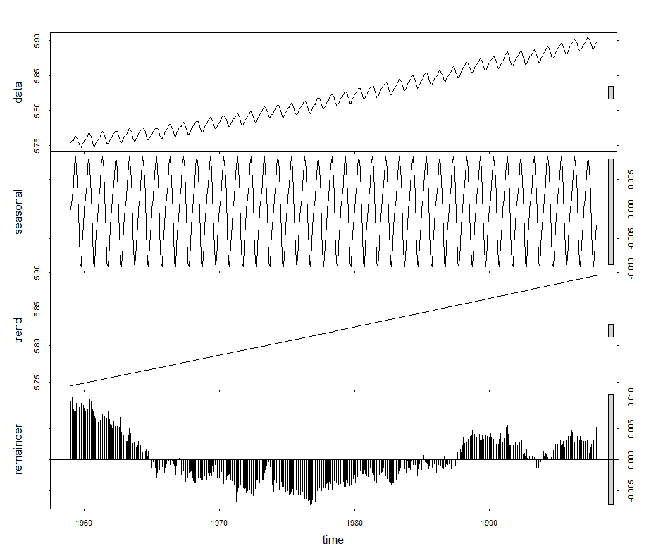
 Figure 8. Keeling CO2 concentration curve at Mauna Loa, Hawaii, showing original data and its decomposition into three parts, a sinusoidal annual variation, a linear trend, and a stochastic residual.
[/caption]
The question is, which component represents the true trend, long term or otherwise? Are linear trends superior to all others? The importance of a trend is tied up with to what use it will be put. A pair of trends, like the sinusoidal and the random residual of the Keeling, might be more important for predicting its short term movements. On the other hand, explicating the long term behavior of the system being measured might feature the large scale linear trend, with the seasonal trend and random variations being but distractions.
Consider the global surface temperature anomalies of Figure 5 again. What are some ways of determining trends? First, note that by "trends" what's really meant are slopes. In the case where there are many places to estimate slopes, there are many slopes. When, for example, a slope is estimated by fitting a line to all the points, there's just a single slope such as in Figure 9. Local linear trends can be estimated from pairs of points in differing sizes of neighborhoods, as depicted in Figures 10 and 11. These can be averaged, if you like, to obtain an overall trend.
[caption id="attachment_1099" align="aligncenter" width="440"]
Figure 8. Keeling CO2 concentration curve at Mauna Loa, Hawaii, showing original data and its decomposition into three parts, a sinusoidal annual variation, a linear trend, and a stochastic residual.
[/caption]
The question is, which component represents the true trend, long term or otherwise? Are linear trends superior to all others? The importance of a trend is tied up with to what use it will be put. A pair of trends, like the sinusoidal and the random residual of the Keeling, might be more important for predicting its short term movements. On the other hand, explicating the long term behavior of the system being measured might feature the large scale linear trend, with the seasonal trend and random variations being but distractions.
Consider the global surface temperature anomalies of Figure 5 again. What are some ways of determining trends? First, note that by "trends" what's really meant are slopes. In the case where there are many places to estimate slopes, there are many slopes. When, for example, a slope is estimated by fitting a line to all the points, there's just a single slope such as in Figure 9. Local linear trends can be estimated from pairs of points in differing sizes of neighborhoods, as depicted in Figures 10 and 11. These can be averaged, if you like, to obtain an overall trend.
[caption id="attachment_1099" align="aligncenter" width="440"]
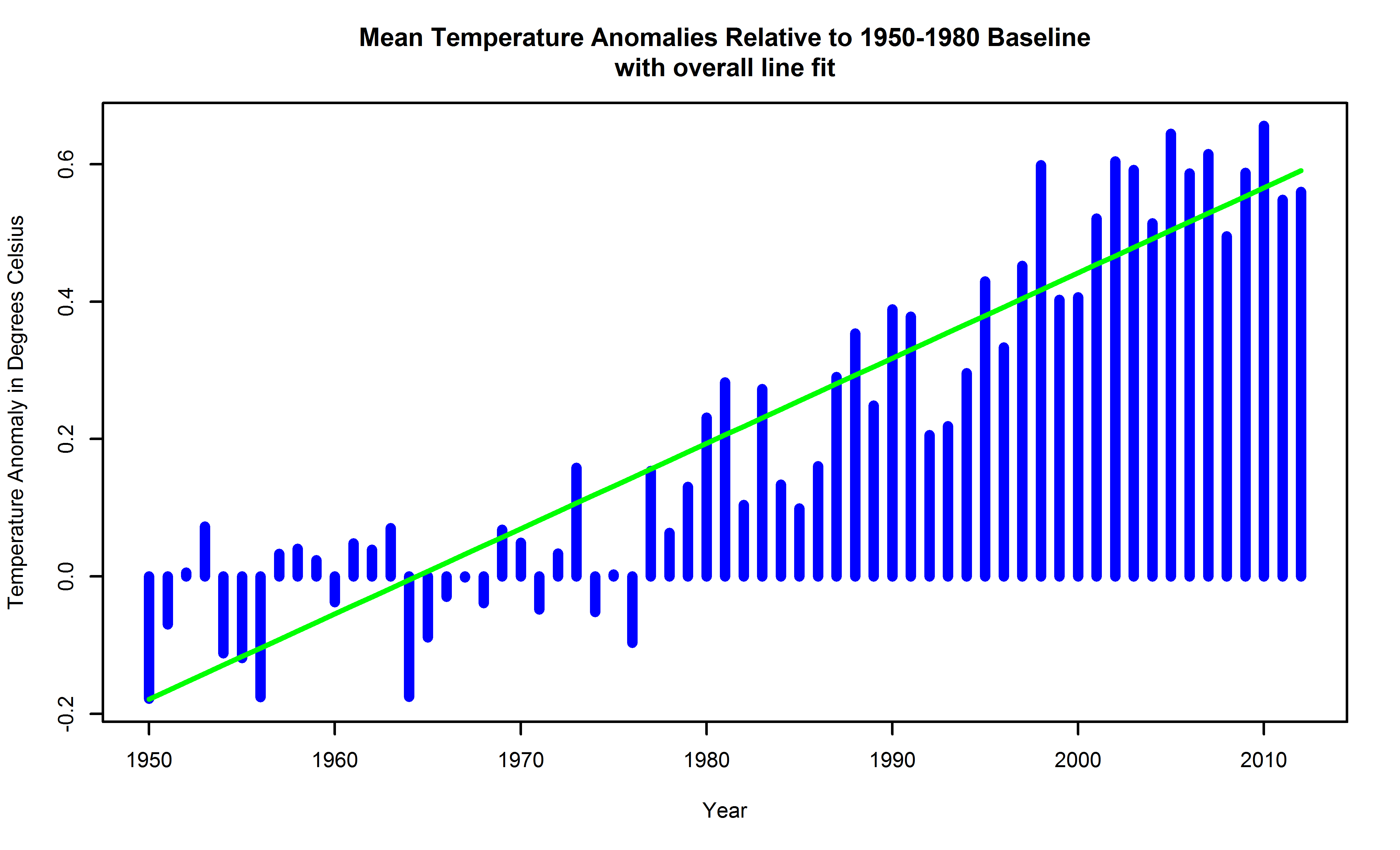 Figure 9. Global surface temperature anomalies relative to a 1950-1980 baseline, with long term linear trend atop.
[/caption]
[caption id="attachment_1096" align="aligncenter" width="440"]
Figure 9. Global surface temperature anomalies relative to a 1950-1980 baseline, with long term linear trend atop.
[/caption]
[caption id="attachment_1096" align="aligncenter" width="440"]
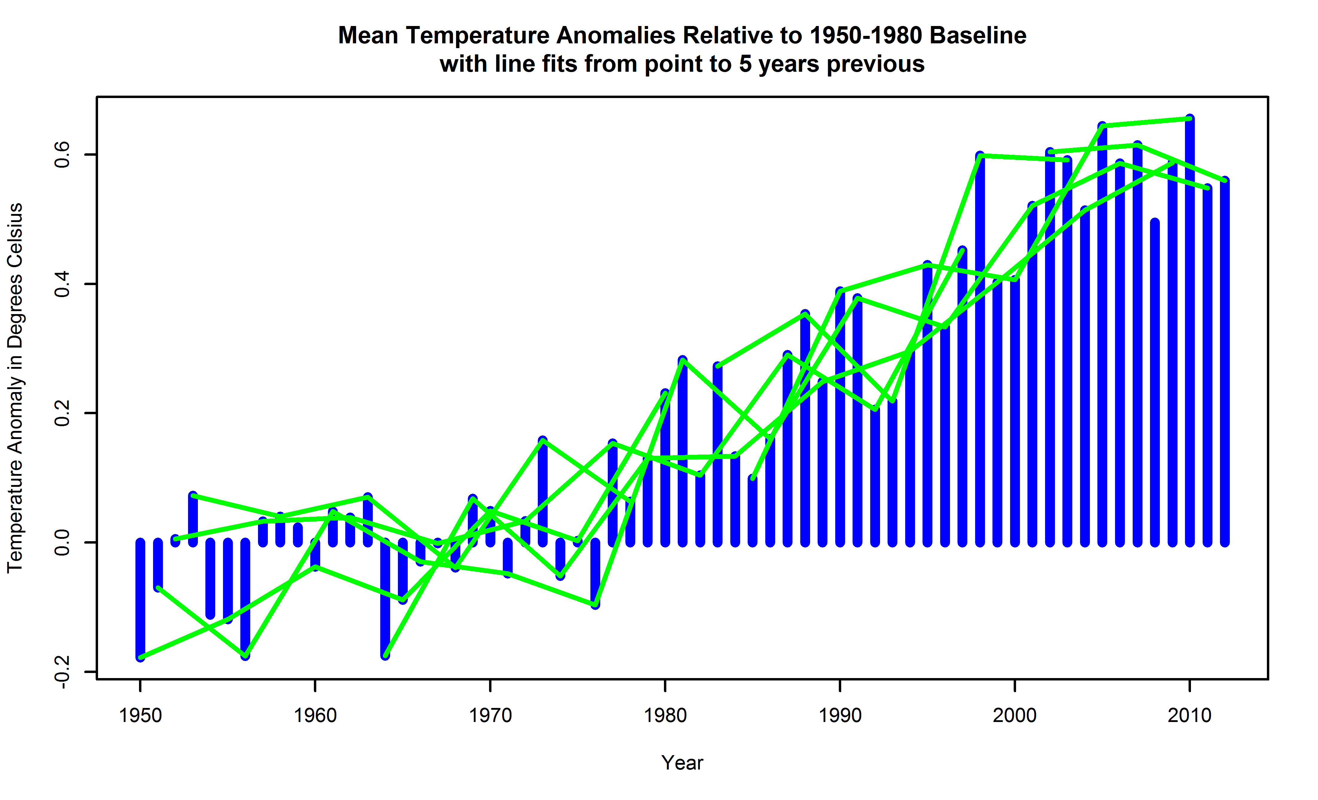 Figure 10. Global surface temperature anomalies relative to a 1950-1980 baseline, with randomly placed trends from local linear having 5 year support atop.
[/caption]
[caption id="attachment_1097" align="aligncenter" width="440"]
Figure 10. Global surface temperature anomalies relative to a 1950-1980 baseline, with randomly placed trends from local linear having 5 year support atop.
[/caption]
[caption id="attachment_1097" align="aligncenter" width="440"]
 Figure 11. Global surface temperature anomalies relative to a 1950-1980 baseline, with randomly placed trends from local linear having 10 year support atop.
[/caption]
Lest the reader think constructing lots of linear trends on varying neighborhoods is somehow crude, note it has a noble history, being used by Boscovich to estimate Earth's ellipticity about 1750, as reported by Koenker.
There is, in addition, a question of what to do if local intervals for fitting the little lines overlap, since these are then (on the face of it) not independent of one another. There are a number of statistical devices for making them independent. One way is to do clever kinds of random sampling from a population of linear trends. Another way is to shrink the intervals until they are infinitesimally small, and, so, necessarily independent. That definition is just the point slope of a curve going through the data, or its first derivative. Numerical methods for estimating these exist---and to the degree they succeed, they obtain estimates of the derivative, even if in doing do they might use finite intervals.
One good way of estimating derivatives involves using a smoothing spline, as sketched in Figure 6, and estimating the derivative(s) of that. Such an estimate of the derivative is shown in Figure 12 where the instantaneous slope is plotted in orange atop the data of Figure 6. The value of the derivative should be read using the scale to the right of the graph. The value to the left shows, as before, temperature anomaly in degrees. The cubic spline itself is plotted in green in that figure. Here it's smoothing parameter is determined by generalized cross-validation, a principled means of taking the subjectivity out of the choice of smoothing parameter. That is explained a bit more in the caption for Figure 12. (See also Cr1979.)
[caption id="attachment_1098" align="aligncenter" width="440"]
Figure 11. Global surface temperature anomalies relative to a 1950-1980 baseline, with randomly placed trends from local linear having 10 year support atop.
[/caption]
Lest the reader think constructing lots of linear trends on varying neighborhoods is somehow crude, note it has a noble history, being used by Boscovich to estimate Earth's ellipticity about 1750, as reported by Koenker.
There is, in addition, a question of what to do if local intervals for fitting the little lines overlap, since these are then (on the face of it) not independent of one another. There are a number of statistical devices for making them independent. One way is to do clever kinds of random sampling from a population of linear trends. Another way is to shrink the intervals until they are infinitesimally small, and, so, necessarily independent. That definition is just the point slope of a curve going through the data, or its first derivative. Numerical methods for estimating these exist---and to the degree they succeed, they obtain estimates of the derivative, even if in doing do they might use finite intervals.
One good way of estimating derivatives involves using a smoothing spline, as sketched in Figure 6, and estimating the derivative(s) of that. Such an estimate of the derivative is shown in Figure 12 where the instantaneous slope is plotted in orange atop the data of Figure 6. The value of the derivative should be read using the scale to the right of the graph. The value to the left shows, as before, temperature anomaly in degrees. The cubic spline itself is plotted in green in that figure. Here it's smoothing parameter is determined by generalized cross-validation, a principled means of taking the subjectivity out of the choice of smoothing parameter. That is explained a bit more in the caption for Figure 12. (See also Cr1979.)
[caption id="attachment_1098" align="aligncenter" width="440"]
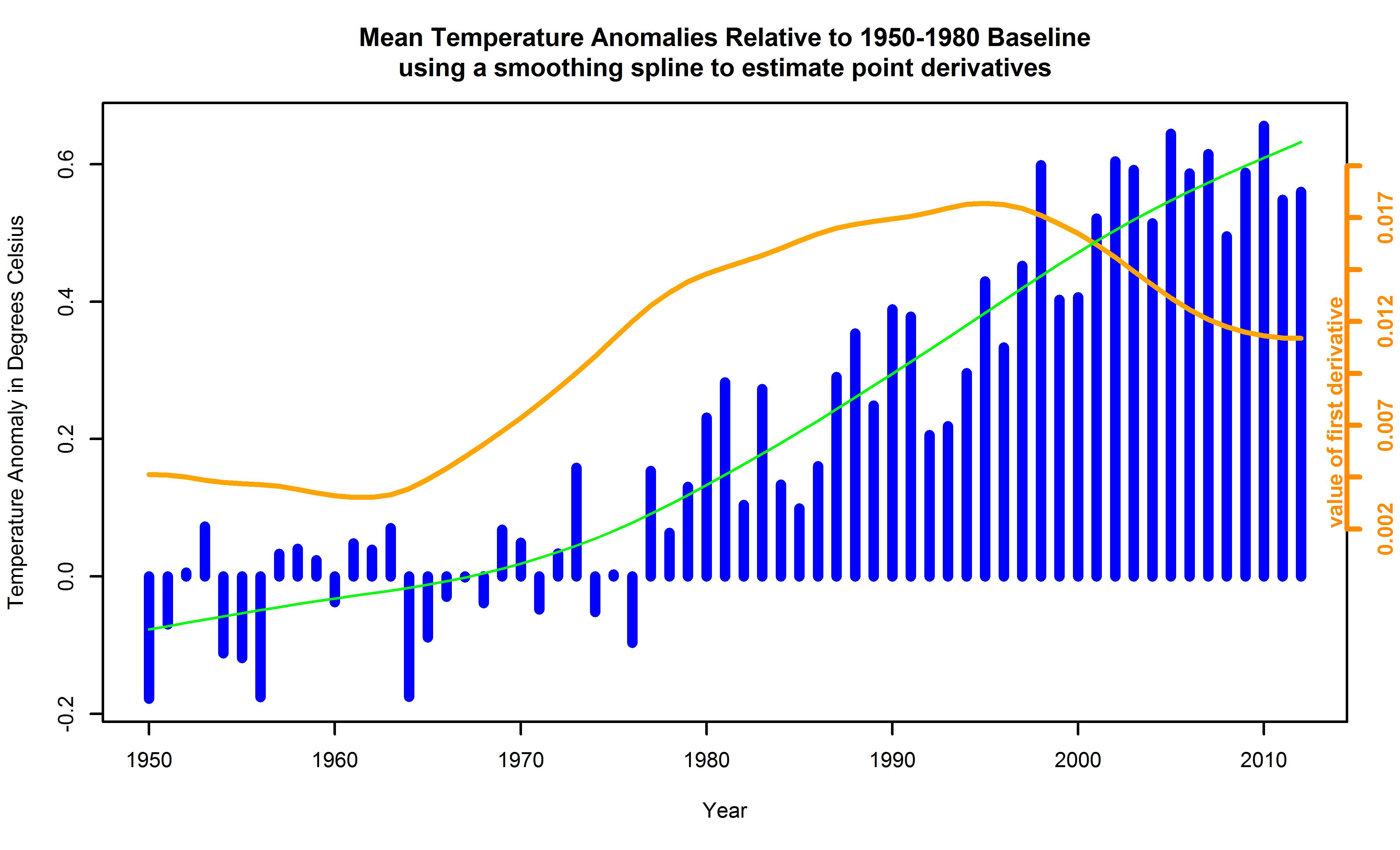 Figure 12. Global surface temperature anomalies relative to a 1950-1980 baseline, with instaneous numerical estimates of derivatives in orange atop, with scale for the derivative to the right of the chart. Note how the value of the first derivative never drops below zero although its magnitude decreases as time approaches 2012. Support for the smoothing spline used to calculate the derivatives is obtained using generalized cross validation. Such cross validation is used to help reduce the possibility that a smoothing parameter is chosen to overfit a particular data set, so the analyst could expect that the spline would apply to as yet uncollected data more than otherwise. Generalized cross validation is a particular clever way of doing that, although it is abstract.
[/caption]
What else might we do?
We could go after a really good approximation to the data of Figure 5. One possibility is to use the Bayesian Rauch-Tung-Striebel ("RTS") smoother to get a good approximation for the underlying curve and estimate the derivatives of that. This is a modification of the famous Kalman filter, the workhorse of much controls engineering and signals work. What that means and how these work is described in an accompanying inset box.
Using the RTS smoother demands variances of the signal be estimated as priors. The larger the ratio of the estimate of the observations variance to the estimate of the process variance is, the smoother the RTS solution. And, yes, as the reader may have guessed, that makes the result dependent upon initial conditions, although hopefully educated initial conditions.
[caption id="attachment_1095" align="aligncenter" width="440"]
Figure 12. Global surface temperature anomalies relative to a 1950-1980 baseline, with instaneous numerical estimates of derivatives in orange atop, with scale for the derivative to the right of the chart. Note how the value of the first derivative never drops below zero although its magnitude decreases as time approaches 2012. Support for the smoothing spline used to calculate the derivatives is obtained using generalized cross validation. Such cross validation is used to help reduce the possibility that a smoothing parameter is chosen to overfit a particular data set, so the analyst could expect that the spline would apply to as yet uncollected data more than otherwise. Generalized cross validation is a particular clever way of doing that, although it is abstract.
[/caption]
What else might we do?
We could go after a really good approximation to the data of Figure 5. One possibility is to use the Bayesian Rauch-Tung-Striebel ("RTS") smoother to get a good approximation for the underlying curve and estimate the derivatives of that. This is a modification of the famous Kalman filter, the workhorse of much controls engineering and signals work. What that means and how these work is described in an accompanying inset box.
Using the RTS smoother demands variances of the signal be estimated as priors. The larger the ratio of the estimate of the observations variance to the estimate of the process variance is, the smoother the RTS solution. And, yes, as the reader may have guessed, that makes the result dependent upon initial conditions, although hopefully educated initial conditions.
[caption id="attachment_1095" align="aligncenter" width="440"]
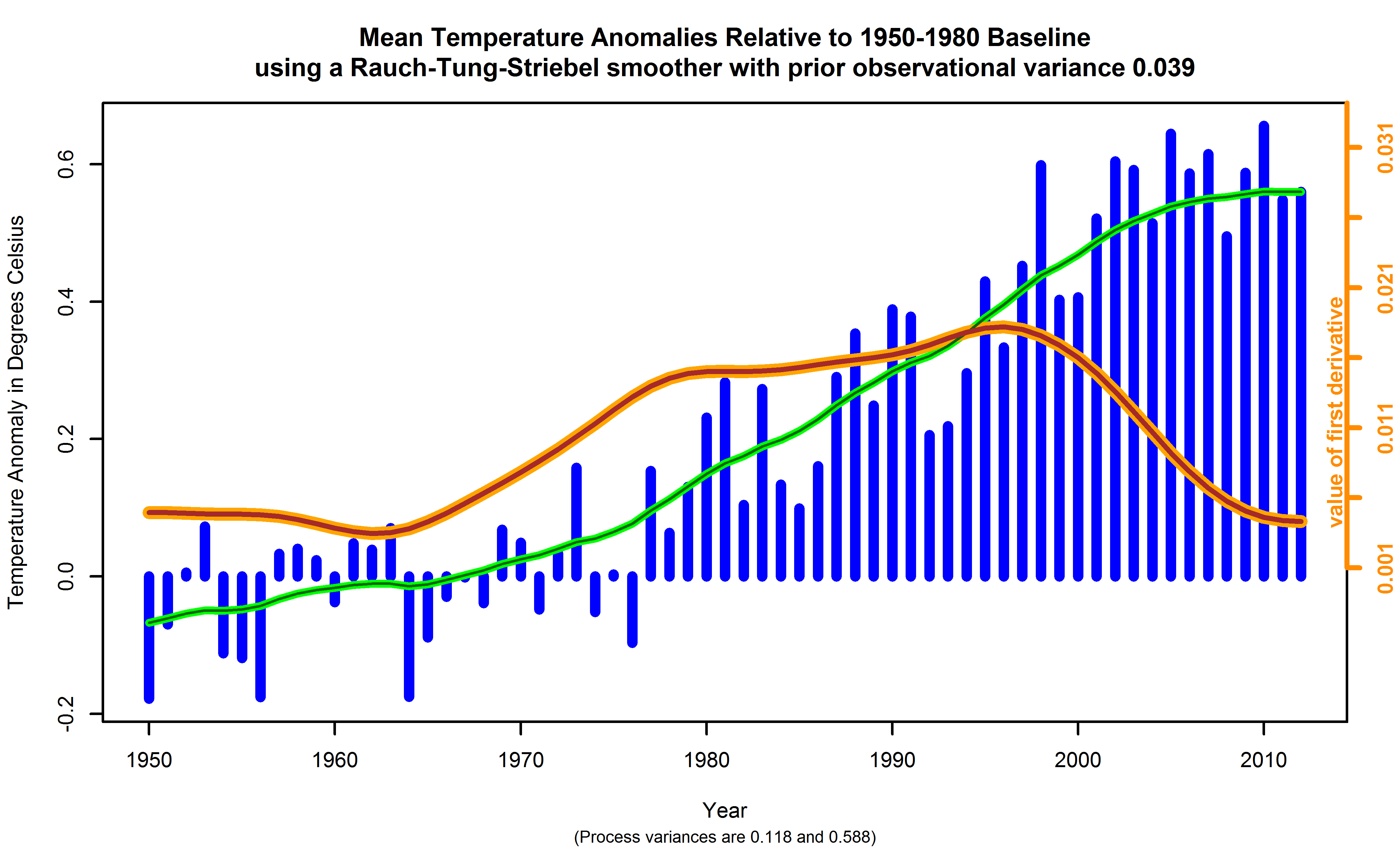 Figure 13. Global surface temperature anomalies relative to a 1950-1980 baseline, with fits using the Rauch-Tung-Striebel smoother placed atop, in green and dark green. The former uses a prior variance of 3 times that of the Figure 5 data corrected for serial correlation. The latter uses a prior variance of 15 times that of the Figure 5 data corrected for serial correlation. The instantaneous numerical estimates of the first derivative derived from the two solutions are shown in orange and brown, respectively, with their scale of values on the right hand side of the chart. Note the two solutions are essentially identical. If compared to the smoothing spline estimate of Figure 12, the derivative has roughly the same shape, but is shifted lower in overall slope, and the drift up and below a mean value is less.
[/caption]
The RTS smoother result for two process variance values of 0.118 ± 002 and high 0.59 ± 0.02 is shown in Figure 13. These are 3 and 15 times the decorrelated variance value for the series of 0.039 ± 0.001, estimated using the long term variance for this series and others like it, corrected for serial correlation. One reason for using two estimates of the process variance is to see how much difference that makes. As can be seen from Figure 13, it does not make much.
Combining all six methods of estimating trends results in Figure 14, which shows the overprinted densities of slopes.
[caption id="attachment_1094" align="aligncenter" width="440"]
Figure 13. Global surface temperature anomalies relative to a 1950-1980 baseline, with fits using the Rauch-Tung-Striebel smoother placed atop, in green and dark green. The former uses a prior variance of 3 times that of the Figure 5 data corrected for serial correlation. The latter uses a prior variance of 15 times that of the Figure 5 data corrected for serial correlation. The instantaneous numerical estimates of the first derivative derived from the two solutions are shown in orange and brown, respectively, with their scale of values on the right hand side of the chart. Note the two solutions are essentially identical. If compared to the smoothing spline estimate of Figure 12, the derivative has roughly the same shape, but is shifted lower in overall slope, and the drift up and below a mean value is less.
[/caption]
The RTS smoother result for two process variance values of 0.118 ± 002 and high 0.59 ± 0.02 is shown in Figure 13. These are 3 and 15 times the decorrelated variance value for the series of 0.039 ± 0.001, estimated using the long term variance for this series and others like it, corrected for serial correlation. One reason for using two estimates of the process variance is to see how much difference that makes. As can be seen from Figure 13, it does not make much.
Combining all six methods of estimating trends results in Figure 14, which shows the overprinted densities of slopes.
[caption id="attachment_1094" align="aligncenter" width="440"]
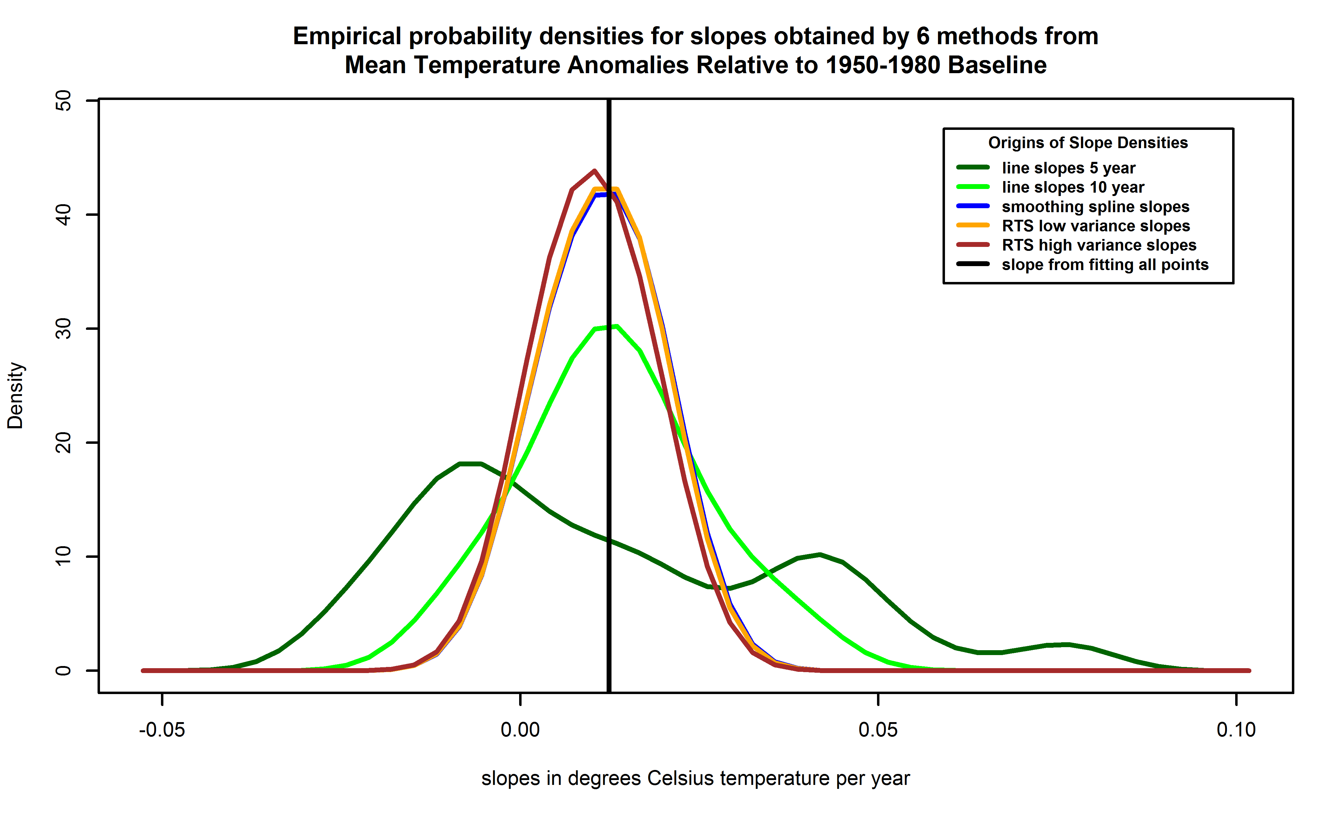 Figure 14. Empirical probability density functions for slopes of temperatures versus years, from each of 6 methods. Empirical probability densities are obtained using kernel density estimation and are preferred to histograms by statisticians because the latter can distort the density due to bin size and boundary effects. Lines correspond to local linear fits with 5 years separation (dark green trace), the local linear fits with 10 years separation (green trace), the smoothing spline (blue trace), the RTS smoother with variance 3 times the corrected estimate for the data as the prior variance (orange trace, mostly hidden by brown trace), and the RTS smoother with 15 times the corrected estimate for the data (brown trace). The blue trace can barely be seen because the RTS smoother with the 3 times variance lies nearly atop of it. The slope value for a linear fit to all the points is also shown (the vertical black line).
[/caption]
Note the spread of possibilities given by the 5 year local linear fits. The 10 year local linear fits, the spline, and the RTS smoother fits have their mode in the vicinity of the overall slope. The 10 year local linear fits slope has broader support, meaning it admits more negative slopes in the range of temperature anomalies observed. The RTS smoother results have peaks slightly below those for the spline, the 10 year local linear fits, and the overall slope. The kernel density estimator allows the possibility of probability mass below zero, even though the spline, and two RTS smoother fits never exhibit slopes below zero. This is a Bayesian-like estimator, since the prior is the real line.
Local linear fits to HadCRUT4 time series were used by Fyfe, Gillet, and Zwiers in their 2013 paper and supplement. We do not know the computational details of those trends, since they were not published, possibly due to Nature Climate Change page count restrictions. Those details matter. From these calculations, which, admittedly, are not as comprehensive as those by Fyfe, Gillet, and Zwiers, we see that robust estimators of trends in temperature during the observational record show these are always positive, even if the magnitudes vary. The RTS smoother solutions suggest slopes in recent years are near zero, providing a basis for questioning whether or not there is a warming "hiatus".
Figure 14. Empirical probability density functions for slopes of temperatures versus years, from each of 6 methods. Empirical probability densities are obtained using kernel density estimation and are preferred to histograms by statisticians because the latter can distort the density due to bin size and boundary effects. Lines correspond to local linear fits with 5 years separation (dark green trace), the local linear fits with 10 years separation (green trace), the smoothing spline (blue trace), the RTS smoother with variance 3 times the corrected estimate for the data as the prior variance (orange trace, mostly hidden by brown trace), and the RTS smoother with 15 times the corrected estimate for the data (brown trace). The blue trace can barely be seen because the RTS smoother with the 3 times variance lies nearly atop of it. The slope value for a linear fit to all the points is also shown (the vertical black line).
[/caption]
Note the spread of possibilities given by the 5 year local linear fits. The 10 year local linear fits, the spline, and the RTS smoother fits have their mode in the vicinity of the overall slope. The 10 year local linear fits slope has broader support, meaning it admits more negative slopes in the range of temperature anomalies observed. The RTS smoother results have peaks slightly below those for the spline, the 10 year local linear fits, and the overall slope. The kernel density estimator allows the possibility of probability mass below zero, even though the spline, and two RTS smoother fits never exhibit slopes below zero. This is a Bayesian-like estimator, since the prior is the real line.
Local linear fits to HadCRUT4 time series were used by Fyfe, Gillet, and Zwiers in their 2013 paper and supplement. We do not know the computational details of those trends, since they were not published, possibly due to Nature Climate Change page count restrictions. Those details matter. From these calculations, which, admittedly, are not as comprehensive as those by Fyfe, Gillet, and Zwiers, we see that robust estimators of trends in temperature during the observational record show these are always positive, even if the magnitudes vary. The RTS smoother solutions suggest slopes in recent years are near zero, providing a basis for questioning whether or not there is a warming "hiatus".
The Rauch-Tung-Striebel smoother is an enhancement of the Kalman filter. Let $latex y_{\kappa}$ denote a set of univariate observations at equally space and successive time steps $latex \kappa$. Describe these as follows:
|
Hiatus periods of 10 to 15 years can arise as a manifestation of internal decadal climate variability, which sometimes enhances and sometimes counteracts the long-term externally forced trend. Internal variability thus diminishes the relevance of trends over periods as short as 10 to 15 years for long-term climate change (Box 2.2, Section 2.4.3). Furthermore, the timing of internal decadal climate variability is not expected to be matched by the CMIP5 historical simulations, owing to the predictability horizon of at most 10 to 20 years (Section 11.2.2; CMIP5 historical simulations are typically started around nominally 1850 from a control run). However, climate models exhibit individual decades of GMST trend hiatus even during a prolonged phase of energy uptake of the climate system (e.g., Figure 9.8; Easterling and Wehner, 2009; Knight et al., 2009), in which case the energy budget would be balanced by increasing subsurface-ocean heat uptake (Meehl et al., 2011, 2013a; Guemas et al., 2013). Owing to sampling limitations, it is uncertain whether an increase in the rate of subsurface-ocean heat uptake occurred during the past 15 years (Section 3.2.4). However, it is very likely that the climate system, including the ocean below 700 m depth, has continued to accumulate energy over the period 1998-2010 (Section 3.2.4, Box 3.1). Consistent with this energy accumulation, global mean sea level has continued to rise during 1998-2012, at a rate only slightly and insignificantly lower than during 1993-2012 (Section 3.7). The consistency between observed heat-content and sea level changes yields high confidence in the assessment of continued ocean energy accumulation, which is in turn consistent with the positive radiative imbalance of the climate system (Section 8.5.1; Section 13.3, Box 13.1). By contrast, there is limited evidence that the hiatus in GMST trend has been accompanied by a slower rate of increase in ocean heat content over the depth range 0 to 700 m, when comparing the period 2003-2010 against 1971-2010. There is low agreement on this slowdown, since three of five analyses show a slowdown in the rate of increase while the other two show the increase continuing unabated (Section 3.2.3, Figure 3.2). [Emphasis added by author.] During the 15-year period beginning in 1998, the ensemble of HadCRUT4 GMST trends lies below almost all model-simulated trends (Box 9.2 Figure 1a), whereas during the 15-year period ending in 1998, it lies above 93 out of 114 modelled trends (Box 9.2 Figure 1b; HadCRUT4 ensemble-mean trend $latex 0.26\,^{\circ}\mathrm{C}$ per decade, CMIP5 ensemble-mean trend $latex 0.16\,^{\circ}\mathrm{C}$ per decade). Over the 62-year period 1951-2012, observed and CMIP5 ensemble-mean trends agree to within $latex 0.02\,^{\circ}\mathrm{C}$ per decade (Box 9.2 Figure 1c; CMIP5 ensemble-mean trend $latex 0.13\,^{\circ}\mathrm{C}$ per decade). There is hence very high confidence that the CMIP5 models show long-term GMST trends consistent with observations, despite the disagreement over the most recent 15-year period. Due to internal climate variability, in any given 15-year period the observed GMST trend sometimes lies near one end of a model ensemble (Box 9.2, Figure 1a, b; Easterling and Wehner, 2009), an effect that is pronounced in Box 9.2, Figure 1a, because GMST was influenced by a very strong El Niño event in 1998. [Emphasis added by author.]The contributions of Fyfe, Gillet, and Zwiers ("FGZ") are to (a) pin down this behavior for a 20 year period using the HadCRUT4 data, and, to my mind, more importantly, (b) to develop techniques for evaluating runs of ensembles of climate models like the CMIP5 suite without commissioning specific runs for the purpose. This, if it were to prove out, would be an important experimental advance, since climate models demand expensive and extensive hardware, and the number of people who know how to program and run them is very limited, possibly a more limiting practical constraint than the hardware. This is the beginning of a great story, I think, one which both advances an understanding of how our experience of climate is playing out, and how climate science is advancing. FGZ took a perfectly reasonable approach and followed it to its logical conclusion, deriving an inconsistency. There's insight to be won resolving it. FGZ try to explicitly model trends due to internal variability. They begin with two equations:
 Figure 15. Figure 1 from Fyfe, Gillet, Zwiers.[/caption]
Why are climate models so less precise than HadCRUT4 observations? Moreover, why do climate models disagree with one another so dramatically? We cannot tell without getting into CMIP5 details, but the same result could be obtained if the climate models came in three Gaussian populations, each with a variance 1.5x that of the observations, but mixed together. We could also obtain the same result if, for some reason, the variance of HadCRUT4 was markedly understated.
That brings us back to the comments about HadCRUT4 made at the end of Section 3. HadCRUT4 is noted for "drop outs" in observations, where either the quality of an observation on a patch of Earth was poor or the observation was missing altogether for a certain month in history. (To be fair, both GISS and BEST have months where there is no data available, especially in early years of the record.) It also has incomplete coverage [Co2013]. Whether or not values for patches are imputed in some way, perhaps using spatial kriging, or whether or not supports to calculate trends are adjusted to avoid these omissions are decisions in use of these data which are critical to resolving the question [Co2013, Gl2011].
As seen in Section 5, what trends you get depends a lot on how they are done. FGZ did linear trends. These are nice because means of trends have simple relationships with the trends themselves. On the other hand, confining trend estimation to local linear trends binds these estimates to being only supported by pairs of actual samples, however sparse these may be. This has the unfortunate effect of producing a broadly spaced set of trends which, when averaged, appear to be a single, tight distribution, close to the vertical black line of Figure 14, but erasing all the detail available by estimating the density of trends with a robust function of the first time derivative of the series. FGZ might be improved by using such, repairing this drawback and also making it more robust against HadCRUT4's inescapable data drops. As mentioned before, however, we really cannot know, because details of their calculations are not available. (Again, this author suspects this fault lies not with FGZ but a matter of page limits.)
In fact, that was indicated by a recent paper from Cowtan and Way, arguing that the limited coverage of HadCRUT4 might explain the discrepancy Fyfe, Gillet, and Zwiers found. In return Fyfe and Gillet argued that even admitting the corrections for polar regions which Cowtan and Way indicate, the CMIP5 models fall short in accounting for global mean surface temperatures. What could be wrong?
Figure 15. Figure 1 from Fyfe, Gillet, Zwiers.[/caption]
Why are climate models so less precise than HadCRUT4 observations? Moreover, why do climate models disagree with one another so dramatically? We cannot tell without getting into CMIP5 details, but the same result could be obtained if the climate models came in three Gaussian populations, each with a variance 1.5x that of the observations, but mixed together. We could also obtain the same result if, for some reason, the variance of HadCRUT4 was markedly understated.
That brings us back to the comments about HadCRUT4 made at the end of Section 3. HadCRUT4 is noted for "drop outs" in observations, where either the quality of an observation on a patch of Earth was poor or the observation was missing altogether for a certain month in history. (To be fair, both GISS and BEST have months where there is no data available, especially in early years of the record.) It also has incomplete coverage [Co2013]. Whether or not values for patches are imputed in some way, perhaps using spatial kriging, or whether or not supports to calculate trends are adjusted to avoid these omissions are decisions in use of these data which are critical to resolving the question [Co2013, Gl2011].
As seen in Section 5, what trends you get depends a lot on how they are done. FGZ did linear trends. These are nice because means of trends have simple relationships with the trends themselves. On the other hand, confining trend estimation to local linear trends binds these estimates to being only supported by pairs of actual samples, however sparse these may be. This has the unfortunate effect of producing a broadly spaced set of trends which, when averaged, appear to be a single, tight distribution, close to the vertical black line of Figure 14, but erasing all the detail available by estimating the density of trends with a robust function of the first time derivative of the series. FGZ might be improved by using such, repairing this drawback and also making it more robust against HadCRUT4's inescapable data drops. As mentioned before, however, we really cannot know, because details of their calculations are not available. (Again, this author suspects this fault lies not with FGZ but a matter of page limits.)
In fact, that was indicated by a recent paper from Cowtan and Way, arguing that the limited coverage of HadCRUT4 might explain the discrepancy Fyfe, Gillet, and Zwiers found. In return Fyfe and Gillet argued that even admitting the corrections for polar regions which Cowtan and Way indicate, the CMIP5 models fall short in accounting for global mean surface temperatures. What could be wrong?
Accordingly, the dispersion of a forecast ensemble can at best only approximate the [probability density function] of forecast uncertainty ... In particular, a forecast ensemble may reflect errors both in statistical location (most or all ensemble members being well away from the actual state of the atmosphere, but relatively nearer to each other) and dispersion (either under- or overrepresenting the forecast uncertainty). Often, operational ensemble forecasts are found to exhibit too little dispersion ..., which leads to overconfidence in probability assessment if ensemble relative frequencies are interpreted as estimating probabilities.In fact, the IPCC reference, Toth, Palmer and others raise the same caution. It could be that the answer to why the variance of the observational data in the Fyfe, Gillet, and Zwiers graph depicted in Figure 15 is so small is that ensemble spread does not properly reflect the true probability density function of the joint distribution of temperatures across Earth. These might be "relatively nearer to each other" than the true dispersion which climate models are accommodating. If Earth's climate is thought of as a dynamical system, and taking note of the suggestion of Kharin that "There is basically one observational record in climate research", we can do the following thought experiment. Suppose the total state of the Earth's climate system can be captured at one moment in time, no matter how, and the climate can be reinitialized to that state at our whim, again no matter how. What happens if this is done several times, and then the climate is permitted to develop for, say, exactly 100 years on each "run"? What are the resulting states? Also suppose the dynamical "inputs" from the Sun, as a function of time, are held identical during that 100 years, as are dynamical inputs from volcanic forcings, as are human emissions of greenhouse gases. Are the resulting states copies of one another? No. Stochastic variability in the operation of climate means these end states will be each somewhat different than one another. Then of what use is the "one observation record"? Well, it is arguably better than no observational record. And, in fact, this kind of variability is a major part of the "internal variability" which is often cited in these literature, including by FGZ. Setting aside the problems of using local linear trends, FGZ's bootstrap approach to the HadCRUT4 ensemble is an attempt to imitate these various runs of Earth's climate. The trouble is, the frequentist bootstrap can only replicate values of observations actually seen. (See inset.) In this case, these replications are those of the HadCRUT4 ensembles. It will never produce values in-between and, as the parameters of temperature anomalies are in general continuous measures, allowing for in-between values seems a reasonable thing to do. No algorithm can account for a dispersion which is not reflected in the variability of the ensemble. If the dispersion of HadCRUT4 is too small, it could be corrected using ensemble MOS methods (Section 7.7.1.) In any case, underdispersion could explain the remarkable difference in variances of populations seen in Figure 15. I think there's yet another way. Consider equations (6.1) and (6.2) again. Recall, here, $latex i$ denotes the $latex i^{th}$ model and $latex j$ denotes the $latex j^{th}$ run of model $latex i$. Instead of $latex k$, however, a bootstrap resampling of the HadCRUT4 ensembles, let $latex \omega$ run over all the 100 ensemble members provided, let $latex \xi$ run over the 2592 patches on Earth's surface, and let $latex \kappa$ run over the 1967 monthly time steps. Reformulate equations (6.1) and (6.2), instead, as
| TEMPERATURE TRENDS | |
|---|---|
| 1997-2012 | |
| Source | Warming ($latex ^{\circ}\,\mathrm{C}$/decade) |
| Climate models | 0.102-0.412 |
| NASA data set | 0.080 |
| HadCRUT data set | 0.046 |
| Cowtan/Way | 0.119 |
| Table 1. Getting warmer. New method brings measured temperatures closer to projections. Added in quotation: "Climate models" refers to the CMIP5 series. "NASA data set" is GISS. "HadCRUT data set" is HadCRUT4. "Cowtan/Way" is from their paper. Note values are per decade, not per year. |
| The bootstrap is a general name for a resampling technique, most commonly associated with what is more properly called the frequentist bootstrap. Given a sample of observations, $latex \mathring{Y} = \{y_{1}, y_{2}, \dots, y_{n}\}$, the bootstrap principle says that in a wide class of statistics and for certain minimum sizes of $latex n$, the sampling density of a statistic $latex h(Y)$ from a population of all $latex Y$, where $latex \mathring{Y}$ is a single observation, can be approximated by the following procedure. Sample $latex \mathring{Y}$ $latex M$ times with replacement to obtain $latex M$ samples each of size $latex n$ called $latex \tilde{Y}_{k}$, $latex k = 1, \dots, M$. For each $latex \tilde{Y}_{k}$, calculate $latex h(\tilde{Y}_{k})$ so as to obtain $latex H = h_{1}, h_{2}, \dots, h_{M}$. The set $latex H$ so obtained is an approximation of the sampling density of $latex h(Y)$ from a population of all $latex Y$. Note that because $latex \mathring{Y}$ is sampled, only elements of that original set of observations will ever show up in any $latex \tilde{Y}_{k}$. This is true even if $latex Y$ is drawn from an interval of the real numbers. This is where a Bayesian bootstrap might be more suitable. In a Bayesian bootstrap, the set of possibilities to be sampled are specified using a prior distribution on $latex Y$ [Da2009, Section 10.5]. A specific observation of $latex Y$, like $latex \mathring{Y}$, is use to update the probability density on $latex Y$, and then values from $latex Y$ are drawn in proportion to this updated probability. Thus, values in $latex Y$ never in $latex \mathring{Y}$ might be drawn. Both bootstraps will, under similar conditions, preserve the sampling distribution of $latex Y$. |