joint with Dara O Shayda Emboldened by our experiments in El Niño analysis and prediction, people in the Azimuth Code Project have been starting to analyze weather and climate data. A lot of this work is exploratory, with no big conclusions. But it's still interesting! So, let's try some blog articles where we present this work. This one will be about the air pressure on the island of Tahiti and in a city called Darwin in Australia: how they're correlated, and how each one varies. This article will also be a quick introduction to some basic statistics, as well as 'continuous wavelet transforms'.

Darwin, Tahiti and El Niños

The El Niño Southern Oscillation is often studied using the air pressure in Darwin, Australia versus the air pressure in Tahiti. When there's an El Niño, it gets stormy in the eastern Pacific so the air temperatures tend to be lower in Tahiti and higher in Darwin. When there's a La Niña, it's the other way around:

The Southern Oscillation Index or SOI is a normalized version of the monthly mean air pressure anomaly in Tahiti minus that in Darwin. Here anomaly means we subtract off the mean, and normalized means that we divide by the standard deviation. So, the SOI tends to be negative when there's an El Niño. On the other hand, when there's an El Niño the Niño 3.4 index tends to be positive—this says it's hotter than usual in a certain patch of the Pacific. Here you can see how this works:

When the Niño 3.4 index is positive, the SOI tends to be negative, and vice versa! It might be fun to explore precisely how well correlated they are. You can get the data to do that by clicking on the links above. But here's another question: how similar are the air pressure anomalies in Darwin and in Tahiti? Do we really need to take their difference, or are they so strongly anticorrelated that either one would be enough to detect an El Niño? You can get the data to answer such questions here: • Southern Oscillation Index based upon annual standardization, Climate Analysis Section, NCAR/UCAR. This includes links to monthly sea level pressure anomalies in Darwin and Tahiti, in either ASCII format (click the second two links) or netCDF format (click the first one and read the explanation). In fact this website has some nice graphs already made, which I might as well show you! Here's the SOI and also the sum of the air pressure anomalies in Darwin and Tahiti, normalized in some way:

(Click to enlarge.) If the sum were zero, the air pressure anomalies in Darwin and Tahiti would contain the same information and life would be simple. But it's not! How similar in character are the air pressure anomalies in Darwin and Tahiti? There are many ways to study this question. Dara tackled it by taking the air pressure anomaly data from 1866 to 2012 and computing some 'continuous wavelet transforms' of these air pressure anomalies. This is a good excuse for explaining how a continuous wavelet transform works.

Very basic statistics

It helps to start with some very basic statistics. Suppose you have a list of numbers $latex x = (x_1, \dots, x_n) $ You probably know how to take their mean, or average. People often write this with angle brackets: $latex \langle x \rangle = \frac{1}{n} \sum_{i = 1}^n x_i $ You can also calculate the mean of their squares: $latex \langle x^2 \rangle = \frac{1}{n} \sum_{i = 1}^n x_i^2 $ If you were naive you might think $latex \langle x^2 \rangle = \langle x \rangle^2,$ but in fact we have: $latex \langle x^2 \rangle \ge \langle x \rangle^2 $ and they're equal only if all the $latex x_i$ are the same. The point is that if the numbers $latex x_i$ are spread out, the squares of the big ones (positive or negative) contribute more to the average of the squares than if we had averaged them out before squaring. The difference $latex \langle x^2 \rangle - \langle x \rangle^2 $ is called the variance; it says how spread out our numbers are. The square root of the variance is the standard deviation: $latex \sigma_x = \sqrt{\langle x^2 \rangle - \langle x \rangle^2 } $ and this has the slight advantage that if you multiply all the numbers $latex x_i$ by some constant $latex c,$ the standard deviation gets multiplied by $latex |c|$. (The variance gets multiplied by $latex c^2$.) We can generalize the variance to a situation where we have two lists of numbers: $latex x = (x_1, \dots, x_n) $ $latex y = (y_1, \dots, y_n) $ Namely, we can form the covariance $latex \langle x y \rangle - \langle x \rangle \langle y \rangle $ This reduces to the variance when $latex x = y$. It measures how much $latex x$ and $latex y$ vary together — 'hand in hand', as it were. A bit more precisely: if $latex x_i$ is greater than its mean value mainly for $latex i$ such that $latex y_i$ is greater than its mean value, the covariance is positive. On the other hand, if $latex x_i$ tends to be greater than average when $latex y_i$ is smaller than average — like with the air pressures at Darwin and Tahiti — the covariance will be negative. For example, if $latex x = (1,-1), \quad y = (1,-1) $ then they 'vary hand in hand', and the covariance $latex \langle x y \rangle - \langle x \rangle \langle y \rangle = 1 - 0 = 1 $ is positive. But if $latex x = (1,-1), \quad y = (-1,1) $ then one is positive when the other is negative, so the covariance $latex \langle x y \rangle - \langle x \rangle \langle y \rangle = -1 - 0 = -1 $ is negative. Of course the covariance will get bigger if we multiply both $latex x$ and $latex y$ by some big number. If we don't want this effect, we can normalize the covariance and get the correlation: $latex \frac{ \langle x y \rangle - \langle x \rangle \langle y \rangle }{\sigma_x \sigma_y} $ which will always be between $latex -1$ and $latex 1$. Okay, we're almost ready for continuous wavelet transforms! If the mean of either $latex x$ or $latex y$ is zero, the formula for covariance simplifies a lot, to $latex \langle x y \rangle = \frac{1}{n} \sum_{i = 1}^n x_i y_i $ So, this quantity says how much the numbers $latex x_i$ 'vary hand in hand' with the numbers $latex y_i,$ in the special case when one (or both) has mean zero. We can do something similar if $latex x, y : \mathbb{R} \to \mathbb{R}$ are functions of time defined for all real numbers $latex t$. The sum becomes an integral, and we have to give up on dividing by $latex n$. We get: $latex \int_{-\infty}^\infty x(t) y(t)\; d t $ This is called the inner product of the functions $latex x$ and $latex y,$ and often it's written $latex \langle x, y \rangle,$ but it's a lot like the covariance.

Continuous wavelet transforms

What are continuous wavelet transforms, and why should we care? People have lots of tricks for studying 'signals', like series of numbers $latex x_i$ or functions $latex x : \mathbb{R} \to \mathbb{R}$. One method is to 'transform' the signal in a way that reveals useful information. The Fourier transform decomposes a signal into sines and cosines of different frequencies. This lets us see how much power the signal has at different frequencies, but it doesn't reveal how the power at different frequencies changes with time. For that we should use something else, like the Gabor transform explained by Blake Pollard in a previous post. Sines and cosines are great, but we might want to look for other patterns in a signal. A 'continuous wavelet transform' lets us scan a signal for appearances of a given pattern at different times and also at different time scales: a pattern could go by quickly, or in a stretched out slow way. To implement the continuous wavelet transform, we need a signal and a pattern to look for. The signal could be a function $latex x : \mathbb{R} \to \mathbb{R}$. The pattern would then be another function $latex y: \mathbb{R} \to \mathbb{R},$ usually called a wavelet. 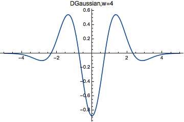Here's an example of a wavelet:

If we're in a relaxed mood, we could call any function that looks like a bump with wiggles in it a wavelet. There are lots of famous wavelets, but this particular one is the fourth derivative of a certain Gaussian. Mathematica calls this particular wavelet DGaussianWavelet[4], and you can look up the formula under 'Details' on their webpage. However, the exact formula doesn't matter at all now! If we call this wavelet $latex y,$ all that matters is that it's a bump with wiggles on it, and that its mean value is 0, or more precisely: $latex \int_{-\infty}^\infty y(t) \; d t = 0 $ As we saw in the last section, this fact lets us take our function $latex x$ and the wavelet $latex y$ and see how much they 'vary hand it hand' simply by computing their inner product: $latex \langle x , y \rangle = \int_{-\infty}^\infty x(t) y(t)\; d t $ Loosely speaking, this measures the 'amount of $latex y$-shaped wiggle in the function $latex x$'. It's amazing how hard it is to say something in plain English that perfectly captures the meaning of a simple formula like the above one—so take the quoted phrase with a huge grain of salt. But it gives a rough intuition. Our wavelet $latex y$ happens to be centered at $latex t = 0$. However, we might be interested in $latex y$-shaped wiggles that are centered not at zero but at some other number $latex s$. We could detect these by shifting the function $latex y$ before taking its inner product with $latex x$: $latex \int_{-\infty}^\infty x(t) y(t-s)\; d t $ We could also be interested in measuring the amount of some stretched-out or squashed version of a $latex y$-shaped wiggle in the function $latex x$. Again we could do this by changing $latex y$ before taking its inner product with $latex x$: $latex \int_{-\infty}^\infty x(t) \; y\left(\frac{t}{P}\right) \; d t $ When $latex P$ is big, we get a stretched-out version of $latex y$. People sometimes call $latex P$ the period, since the period of the wiggles in $latex y$ will be proportional to this (though usually not equal to it). Finally, we can combine these ideas, and compute $latex \int_{-\infty}^\infty x(t) \; y\left(\frac{t- s}{P}\right)\; dt $ This is a function of the shift $latex s$ and period $latex P$ which says how much of the $latex s$-shifted, $latex P$-stretched wavelet $latex y$ is lurking in the function $latex x$. It's a version of the continuous wavelet transform! Mathematica implements this idea for 'time series', meaning lists of numbers $latex x = (x_1,\dots,x_n)$ instead of functions $latex x : \mathbb{R} \to \mathbb{R}$. The idea is that we think of the numbers as samples of a function $latex x$: $latex x_1 = x(\Delta t) $ $latex x_2 = x(2 \Delta t) $ and so on, where $latex \Delta t$ is some time step, and replace the integral above by a suitable sum. Mathematica has a function ContinuousWaveletTransform that does this, giving $latex w(s,P) = \frac{1}{\sqrt{P}} \sum_{i = 1}^n x_i \; y\left(\frac{i \Delta t - s}{P}\right) $ The factor of $latex 1/\sqrt{P}$ in front is a useful extra trick: it's the right way to compensate for the fact that when you stretch out out your wavelet $latex y$ by a factor of $latex P,$ it gets bigger. So, when we're doing integrals, we should define the continuous wavelet transform of $latex y$ by: $latex w(s,P) = \frac{1}{\sqrt{P}} \int_{-\infty}^\infty x(t) y(\frac{t- s}{P})\; dt $

The results

Starting with the air pressure anomaly at Darwin, and taking DGaussianWavelet[4] as his wavelet, Dara Shayda computed the continuous wavelet transform $latex w(s,P)$ as above. To show us the answer, he created a scalogram:

This show roughly how big the continuous wavelet transform $latex w(s,P)$ is for different shifts $latex s$ and periods $latex P$. Blue means it's very small, green means it's bigger, yellow means even bigger and read means very large. Tahiti gave this:

You'll notice that the patterns at Darwin and Tahiti are similar in character, but notably different in detail. For example, the red spots, where our chosen wavelet shows up strongly with period of order ~100 months, occur at different times. Puzzle 1. What is the meaning of the 'spikes' in these scalograms? What sort of signal would give a spike of this sort? Puzzle 2. Do a Gabor transform, also known as a 'windowed Fourier transform', of the same data. Blake Pollard explained the Gabor transform in his article Milankovitch vs the Ice Ages. This is a way to see how much a signal wiggles at a given frequency at a given time: we multiply the signal by a shifted Gaussian and then takes its Fourier transform. Puzzle 3. Read about continuous wavelet transforms. If we want to reconstruct our signal $latex x$ from its continuous wavelet transform, why should we use a wavelet $latex y$ with $latex \int_{-\infty}^\infty y(t) \; d t = 0 ? $ In fact we want a somewhat stronger condition, which is implied by the above equation when the Fourier transform of $latex y$ is smooth and integrable: • Continuous wavelet transform, Wikipedia.

Another way to understand correlations

David Tweed mentioned another approach from signal processing to understanding the quantity $latex \langle x y \rangle = \frac{1}{n} \sum_{i = 1}^n x_i y_i $ If we've got two lists of data $latex x$ and $latex y$ that we want to compare to see if they behave similarly, the first thing we ought to do is multiplicatively scale each one so they're of comparable magnitude. There are various possibilities for assigning a scale, but a reasonable one is to ensure they have equal 'energy' $latex \sum_{i=1}^n x_i^2 = \sum_{i=1}^n y_i^2 $ (This can be achieved by dividing each list by its standard deviation, which is equivalent to what was done in the main derivation above.) Once we've done that then it's clear that looking at $latex \sum_{i=1}^n (x_i-y_i)^2 $ gives small values when they have a very good match and progressively bigger values as they become less similar. Observe that $latex \begin{array}{ccl} \displaystyle{\sum_{i=1}^n (x_i-y_i)^2 } &=& \displaystyle{ \sum_{i=1}^n (x_i^2 - 2 x_i y_i + y_i^2) }\\ &=& \displaystyle{ \sum_{i=1}^n x_i^2 - 2 \sum_{i=1}^n x_i y_i + \sum_{i=1}^n y_i^2 } \end{array} $ Since we've scaled things so that $latex \sum_{i=1}^n x_i^2$ and $latex \sum_{i=1}^n y_i^2$ are constants, we can see that when $latex \sum_{i=1}^n x_i y_i$ becomes bigger, $latex \displaystyle{ \sum_{i=1}^n (x_i-y_i)^2 }$ becomes smaller. So, $latex \displaystyle{\sum_{i=1}^n x_i y_i} $ serves as a measure of how close the lists are, under these assumptions.