

|
|
|
|
A good place to start is this interesting paper:
• Gavin E. Crooks, Measuring thermodynamic length.
which was pointed out by John Furey in a discussion about entropy and uncertainty.
The idea here should work for either classical or quantum statistical mechanics. The paper describes the classical version, so just for a change of pace let me describe the quantum version.
First a lightning review of quantum statistical mechanics. Suppose you have a quantum system with some Hilbert space. When you know as much as possible about your system, then you describe it by a unit vector in this Hilbert space, and you say your system is in a pure state. Sometimes people just call a pure state a 'state'. But that can be confusing, because in statistical mechanics you also need more general 'mixed states' where you don't know as much as possible. A mixed state is described by a density matrix, meaning a positive operator $ \rho$ with trace equal to 1:
$$ \mathrm{tr}(\rho) = 1$$The idea is that any observable is described by a self-adjoint operator $ A$, and the expected value of this observable in the mixed state $ \rho$ is
$$ \langle A \rangle = \mathrm{tr}(\rho A)$$The entropy of a mixed state is defined by
$$ S(\rho) = -\mathrm{tr}(\rho \; \mathrm{ln} \, \rho)$$where we take the logarithm of the density matrix just by taking the log of each of its eigenvalues, while keeping the same eigenvectors. This formula for entropy should remind you of the one that Gibbs and Shannon used — the one I explained a while back.
Back then I told you about the 'Gibbs ensemble': the mixed state that maximizes entropy subject to the constraint that some observable have a given value. We can do the same thing in quantum mechanics, and we can even do it for a bunch of observables at once. Suppose we have some observables $ X_1, \dots, X_n$ and we want to find the mixed state $ \rho$ that maximizes entropy subject to these constraints:
$$ \langle X_i \rangle = x_i $$for some numbers $ x_i$. Then a little exercise in Lagrange multipliers shows that the answer is the Gibbs state:
$$ \rho = \frac{1}{Z} \mathrm{exp}(-\lambda_1 X_1 + \cdots + \lambda_n X_n) $$Huh? 
This answer needs some explanation. First of all, the numbers $ \lambda_1, \dots \lambda_n$ are called Lagrange multipliers. You have to choose them right to get
$$ \langle X_i \rangle = x_i $$So, in favorable cases, they will be functions of the numbers $ x_i$. And when you're really lucky, you can solve for the numbers $ x_i$ in terms of the numbers $ \lambda_i$. We call $ \lambda_i$ the conjugate variable of the observable $ X_i$. For example, the conjugate variable of energy is inverse temperature!
Second of all, we take the exponential of a self-adjoint operator just as we took the logarithm of a density matrix: just take the exponential of each eigenvalue.
(At least this works when our self-adjoint operator has only eigenvalues in its spectrum, not any continuous spectrum. Otherwise we need to get serious and use the functional calculus. Luckily, if your system's Hilbert space is finite-dimensional, you can ignore this parenthetical remark!)
But third: what's that number $ Z$? It begins life as a humble normalizing factor. Its job is to make sure $ \rho$ has trace equal to 1:
$$ Z = \mathrm{tr}(\mathrm{exp}(-\lambda_1 X_1 + \cdots + \lambda_n X_n)) $$However, once you get going, it becomes incredibly important! It's called the partition function of your system.
As an example of what it's good for, it turns out you can compute the numbers $ x_i$ as follows:
$$ x_i = - \frac{\partial}{\partial \lambda_i} \mathrm{ln} Z$$In other words, you can compute the expected values of the observables $ X_i$ by differentiating the log of the partition function:
$$ \langle X_i \rangle = - \frac{\partial}{\partial \lambda_i} \mathrm{ln} Z$$Or in still other words,
$$ \langle X_i \rangle = - \frac{1}{Z} \; \frac{\partial Z}{\partial \lambda_i}$$To believe this you just have to take the equations I've given you so far and mess around — there's really no substitute for doing it yourself. I've done it fifty times, and every time I feel smarter.
But we can go further: after the 'expected value' or 'mean' of an observable comes its variance, which is the square of its standard deviation:
$$ (\Delta A)^2 = \langle A^2 \rangle - \langle A \rangle^2 $$This measures the size of fluctuations around the mean. And in the Gibbs state, we can compute the variance of the observable $ X_i$ as the second derivative of the log of the partition function:
$$ \langle X_i^2 \rangle - \langle X_i \rangle^2 = \frac{\partial^2}{\partial^2 \lambda_i} \mathrm{ln} Z$$Again: calculate and see.
But when we've got lots of observables, there's something better than the variance of each one. There's the covariance matrix of the whole lot of them! Each observable $ X_i$ fluctuates around its mean value $ x_i$... but these fluctuations are not independent! They're correlated, and the covariance matrix says how.
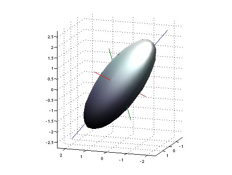
All this is very visual, at least for me. If you imagine the fluctuations as forming a blurry patch near the point $ (x_1, \dots, x_n)$, this patch will be ellipsoidal in shape, at least when all our random fluctuations are Gaussian. And then the shape of this ellipsoid is precisely captured by the covariance matrix! In particular, the eigenvectors of the covariance matrix will point along the principal axes of this ellipsoid, and the eigenvalues will say how stretched out the ellipsoid is in each direction!
To understand the covariance matrix, it may help to start by rewriting the variance of a single observable $ A$ as
$$ (\Delta A)^2 = \langle (A - \langle A \rangle)^2 \rangle $$That's a lot of angle brackets, but the meaning should be clear. First we look at the difference between our observable and its mean value, namely
$$ A - \langle A \rangle$$Then we square this, to get something that's big and positive whenever our observable is far from its mean. Then we take the mean value of the that, to get an idea of how far our observable is from the mean on average.
We can use the same trick to define the covariance of a bunch of observables $ X_i$. We get an $ n \times n$ matrix called the covariance matrix, whose entry in the ith row and jth column is
$$ \langle (X_i - \langle X_i \rangle) (X_j - \langle X_j \rangle) \rangle $$If you think about it, you can see that this will measure correlations in the fluctuations of your observables.
An interesting difference between classical and quantum mechanics shows up here. In classical mechanics the covariance matrix is always symmetric — but not in quantum mechanics! You see, in classical mechanics, whenever we have two observables $ A$ and $ B$, we have
$$ \langle A B \rangle = \langle B A \rangle$$since observables commute. But in quantum mechanics this is not true! For example, consider the position $ q$ and momentum $ p$ of a particle. We have
$$ q p = p q + i $$so taking expectation values we get
$$ \langle q p \rangle = \langle p q \rangle + i $$So, it's easy to get a non-symmetric covariance matrix when our observables $ X_i$ don't commute. However, the real part of the covariance matrix is symmetric, even in quantum mechanics. So let's define
$$ g_{ij} = \mathrm{Re} \langle (X_i - \langle X_i \rangle) (X_j - \langle X_j \rangle) \rangle $$You can check that the matrix entries here are the second derivatives of the partition function:
$$ g_{ij} = \frac{\partial^2}{\partial \lambda_i \partial \lambda_j} \mathrm{ln} Z $$And now for the cool part: this is where information geometry comes in! Suppose that for any choice of values $ x_i$ we have a Gibbs state with
$$ \langle X_i \rangle = x_i $$Then for each point
$$ x = (x_1, \dots , x_n) \in \mathbb{R}^n$$we have a matrix
$$ g_{ij} = \mathrm{Re} \langle (X_i - \langle X_i \rangle) (X_j - \langle X_j \rangle) \rangle = \frac{\partial^2}{\partial \lambda_i \partial \lambda_j} \mathrm{ln} Z $$And this matrix is not only symmetric, it's also positive. And when it's positive definite we can think of it as an inner product on the tangent space of the point $ x$. In other words, we get a Riemannian metric on $ \mathbb{R}^n$. This is called the Fisher information metric.
I hope you can see through the jargon to the simple idea. We've got a space. Each point $ x$ in this space describes the maximum-entropy state of a quantum system for which our observables have specified mean values. But in each of these states, the observables are random variables. They don't just sit at their mean value, they fluctuate! You can picture these fluctuations as forming a little smeared-out blob in our space. To a first approximation, this blob is an ellipsoid. And if we think of this ellipsoid as a 'unit ball', it gives us a standard for measuring the length of any little vector sticking out of our point. In other words, we've got a Riemannian metric: the Fisher information metric!
Now if you look at the Wikipedia article you'll see a more general but to me somewhat scarier definition of the Fisher information metric. This applies whenever we've got a manifold whose points label arbitrary mixed states of a system. But Crooks shows this definition reduces to his — the one I just described — when our manifold is $ \mathbb{R}^n$ and it's parametrizing Gibbs states in the way we've just seen.
More precisely: both Crooks and the Wikipedia article describe the classical story, but it parallels the quantum story I've been telling... and I think the quantum version is well-known. I believe the quantum version of the Fisher information metric is sometimes called the Bures metric, though I'm a bit confused about what the Bures metric actually is.
You can read a discussion of this article on Azimuth, and make your own comments or ask questions there!
|
|
|
|