[Last time](https://forum.azimuthproject.org/discussion/2298/lecture-64-chapter-4-the-category-of-enriched-profunctors) we reached the technical climax of this chapter: constructing the category of enriched profunctors. If you found that difficult, you'll be relieved to hear it's downhill from here on, at least in Chapter 4. We will now apply all our hard work.
One application is to _collaborative design_. Fong and Spivak discuss it in their [the book](http://math.mit.edu/~dspivak/teaching/sp18/7Sketches.pdf), based on this paper by a student of Spivak:
* Andrea Censi, [A mathematical theory of co-design](https://arxiv.org/abs/1512.08055).
Censi's work is based on \\(\textbf{Bool}\\)-enriched profunctors, also known as feasibility relations. We introduced these in [Lecture 56](https://forum.azimuthproject.org/discussion/2280/lecture-56-chapter-4-feasibility-relations/p1).
Remember, a feasibility relation \\( \Phi : X\nrightarrow Y \\) is a monotone function
\[ \Phi : X^{\text{op}} \times Y \to \mathbf{Bool} .\]
If \\( \Phi(x,y) = \text{true}\\), we say **\\(x\\) can be obtained given \\(y\\)**. The idea is that we use elements of \\( X\\) to describe 'requirements' - things you want - and elements of \\(Y\\) to describe 'resources' - things you have.
The idea of Andrea Censi's theory that we can compute the design requirements of a complex system from those of its parts using 'co-design diagrams'. These are really pictures of big complicated feasibility relations, like this:
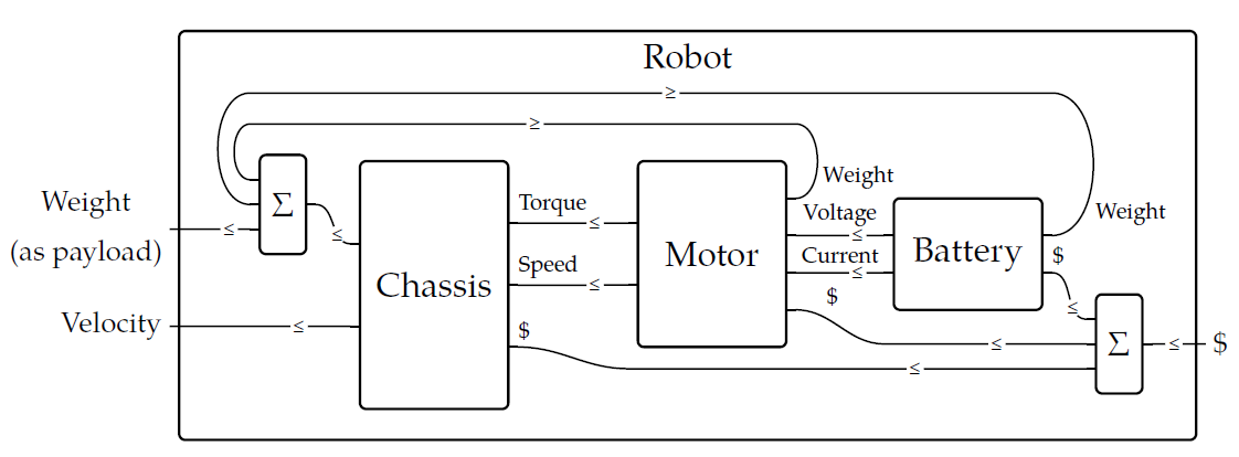 This big complicated feasibility relation is built from simpler ones in various ways. Each wire in this diagram is labeled with the name of a preorder, and each little box is itself a feasibility relation between preorders. We've described how to _compose_ feasibility relations in [Lecture 58](https://forum.azimuthproject.org/discussion/2283/lecture-58-chapter-4-composing-feasibility-relations/p1), and that corresponds to feeding the outputs of one little box into another. But there are other things going on in this picture, like boxes sitting side by side, and wires that bend around backwards! This is what I need to explain - it may take a couple lectures to do this.
Instead of diving into the mathematical details today, let me quote the book's general explanation of the diagram above:
> As an example, consider the design problem of creating a robot to carry some load at some velocity. The top-level planner breaks the problem into three design teams: team chassis, team motor, and team battery. Each of these teams could break up into multiple parts and the process repeated, but let's remain at the top level and consider the resources produced and the resources required by each of our three teams.
> The chassis in some sense provides all the functionality—it carries the load at the velocity—but it requires some things in order to do so. It requires money, of course, but more to the point it requires a source of torque and speed. These are supplied by the motor, which in turn needs voltage and current from the battery. Both the motor and the battery cost money, but more importantly they need to be carried by the chassis: they become part of the load. A feedback loop is created: the chassis must carry all the weight, even that of the parts that power the chassis. A heavier battery might provide more energy to power the chassis, but is the extra power worth the heavier load?
> In the picture, each part—chassis, motor, battery, and robot—is shown as a box with ports on the left and right. The functionalities, or resources produced by the part are on the left of the box, and the resources required by the part are on the right.
> The boxes marked \\(\Sigma\\) correspond to summing inputs. These boxes are not to be designed, but we will see later that they fit easily into the same conceptual framework. Note also the \\(\leq\\)'s on each wire; they indicate that if box \\(A\\) requires a resource that box \\(B\\) produces, then \\(A\\)'s requirement must be less than or equal to \\(B\\)'s production.
Next time we'll get into more detail.
But to wrap up for today, here are few puzzles!
We've been talking about enriched functors and also enriched profunctors. How are they related? The first cool fact is that any enriched functor gives _two_ enriched profunctors: one going each way.
**Puzzle 201.** Show that any \\(\mathcal{V}\\)-enriched functor \\(F: \mathcal{X} \to \mathcal{Y}\\) gives a \\(\mathcal{V}\\)-enriched profunctor
\[ \hat{F} \colon \mathcal{X} \nrightarrow \mathcal{Y} \]
defined by
\[ \hat{F} (x,y) = \mathcal{Y}(F(x), y ) .\]
**Puzzle 202.** Show that any \\(\mathcal{V}\\)-enriched functor \\(F: \mathcal{X} \to \mathcal{Y}\\) gives a \\(\mathcal{V}\\)-enriched profunctor
\[ \check{F} \colon \mathcal{Y} \nrightarrow \mathcal{X} \]
defined by
\[ \check{F} (y,x) = \mathcal{Y}(y,F(x)) .\]
These two constructions have funny names. \\(\hat{F} \colon \mathcal{X} \nrightarrow \mathcal{Y}\\) is called the **companion** of \\(F\\) and \\( \check{F} \colon \mathcal{Y} \nrightarrow \mathcal{X} \\), going back, is called the **conjoint** of \\(F\\).
If you have trouble remembering these, remember that a 'companion' is like a fellow traveler, going the same way as our original functor. The word 'conjoint' should remind you of 'adjoint', which means something going back the other way.
In fact there's a relationship between adjoints and conjoints!
**Puzzle 203.** We say a \\(\mathcal{V}\\)-enriched functor \\(F: \mathcal{X} \to \mathcal{Y}\\) is a **left adjoint** of a \\(\mathcal{V}\\)-enriched functor \\(G: \mathcal{Y} \to \mathcal{X}\\) if
\[ \mathcal{Y}(F(x), y) = \mathcal{X}(x,G(y)) \]
for all objects \\(x\\) of \\(\mathcal{X}\\) and \\(y\\) of \\(\mathcal{Y}\\). In this situation we also say \\(G\\) is the **right adjoint** of \\(F\\). Show that \\(F\\) is the left adjoint of \\(G\\) if and only if
\[ \hat{F} = \check{G} . \]
Pretty!
This big complicated feasibility relation is built from simpler ones in various ways. Each wire in this diagram is labeled with the name of a preorder, and each little box is itself a feasibility relation between preorders. We've described how to _compose_ feasibility relations in [Lecture 58](https://forum.azimuthproject.org/discussion/2283/lecture-58-chapter-4-composing-feasibility-relations/p1), and that corresponds to feeding the outputs of one little box into another. But there are other things going on in this picture, like boxes sitting side by side, and wires that bend around backwards! This is what I need to explain - it may take a couple lectures to do this.
Instead of diving into the mathematical details today, let me quote the book's general explanation of the diagram above:
> As an example, consider the design problem of creating a robot to carry some load at some velocity. The top-level planner breaks the problem into three design teams: team chassis, team motor, and team battery. Each of these teams could break up into multiple parts and the process repeated, but let's remain at the top level and consider the resources produced and the resources required by each of our three teams.
> The chassis in some sense provides all the functionality—it carries the load at the velocity—but it requires some things in order to do so. It requires money, of course, but more to the point it requires a source of torque and speed. These are supplied by the motor, which in turn needs voltage and current from the battery. Both the motor and the battery cost money, but more importantly they need to be carried by the chassis: they become part of the load. A feedback loop is created: the chassis must carry all the weight, even that of the parts that power the chassis. A heavier battery might provide more energy to power the chassis, but is the extra power worth the heavier load?
> In the picture, each part—chassis, motor, battery, and robot—is shown as a box with ports on the left and right. The functionalities, or resources produced by the part are on the left of the box, and the resources required by the part are on the right.
> The boxes marked \\(\Sigma\\) correspond to summing inputs. These boxes are not to be designed, but we will see later that they fit easily into the same conceptual framework. Note also the \\(\leq\\)'s on each wire; they indicate that if box \\(A\\) requires a resource that box \\(B\\) produces, then \\(A\\)'s requirement must be less than or equal to \\(B\\)'s production.
Next time we'll get into more detail.
But to wrap up for today, here are few puzzles!
We've been talking about enriched functors and also enriched profunctors. How are they related? The first cool fact is that any enriched functor gives _two_ enriched profunctors: one going each way.
**Puzzle 201.** Show that any \\(\mathcal{V}\\)-enriched functor \\(F: \mathcal{X} \to \mathcal{Y}\\) gives a \\(\mathcal{V}\\)-enriched profunctor
\[ \hat{F} \colon \mathcal{X} \nrightarrow \mathcal{Y} \]
defined by
\[ \hat{F} (x,y) = \mathcal{Y}(F(x), y ) .\]
**Puzzle 202.** Show that any \\(\mathcal{V}\\)-enriched functor \\(F: \mathcal{X} \to \mathcal{Y}\\) gives a \\(\mathcal{V}\\)-enriched profunctor
\[ \check{F} \colon \mathcal{Y} \nrightarrow \mathcal{X} \]
defined by
\[ \check{F} (y,x) = \mathcal{Y}(y,F(x)) .\]
These two constructions have funny names. \\(\hat{F} \colon \mathcal{X} \nrightarrow \mathcal{Y}\\) is called the **companion** of \\(F\\) and \\( \check{F} \colon \mathcal{Y} \nrightarrow \mathcal{X} \\), going back, is called the **conjoint** of \\(F\\).
If you have trouble remembering these, remember that a 'companion' is like a fellow traveler, going the same way as our original functor. The word 'conjoint' should remind you of 'adjoint', which means something going back the other way.
In fact there's a relationship between adjoints and conjoints!
**Puzzle 203.** We say a \\(\mathcal{V}\\)-enriched functor \\(F: \mathcal{X} \to \mathcal{Y}\\) is a **left adjoint** of a \\(\mathcal{V}\\)-enriched functor \\(G: \mathcal{Y} \to \mathcal{X}\\) if
\[ \mathcal{Y}(F(x), y) = \mathcal{X}(x,G(y)) \]
for all objects \\(x\\) of \\(\mathcal{X}\\) and \\(y\\) of \\(\mathcal{Y}\\). In this situation we also say \\(G\\) is the **right adjoint** of \\(F\\). Show that \\(F\\) is the left adjoint of \\(G\\) if and only if
\[ \hat{F} = \check{G} . \]
Pretty!  **[To read other lectures go here.](http://www.azimuthproject.org/azimuth/show/Applied+Category+Theory#Chapter_4)**