guest post by Eugene Lerman
Hi, I'm Eugene Lerman. I met John back in the mid 1980s when John and I were grad students at MIT. John was doing mathematical physics and I was studying symplectic geometry. We never talked about networks. Now I teach in the math department at the University of Illinois at Urbana, and we occasionally talk about networks on his blog.
A few years ago a friend of mine who studies locomotion in humans and other primates asked me if I knew of any math that could be useful to him.
I remember coming across an expository paper on 'coupled cell networks':
• Martin Golubitsky and Ian Stewart, Nonlinear dynamics of networks: the groupoid formalism, Bull. Amer. Math. Soc. 43 (2006), 305–364.
In this paper, Golubitsky and Stewart used the study of animal gaits and models for the hypothetical neural networks called 'central pattern generators' that give rise to these gaits as motivation for the study of networks of ordinary differential equations with symmetry. In particular they were interested in 'synchrony'. When a horse trots, or canters, or gallops, its limbs move in an appropriate pattern, with different pairs of legs moving in synchrony.
They explained that synchrony (and the patterns) could arise when the differential equations have finite group symmetries. They also proposed several systems of symmetric ODEs that could generate the appropriate patterns.
Later on Golubitsky and Stewart noticed that there are systems of differential equations that have no group symmetries but whose solutions nonetheless exhibit certain synchrony. They found an explanation: these ODEs were 'groupoid invariant'. I thought that it would be fun to understand what 'groupoid invariant' meant and why such invariance leads to synchrony.
I talked my colleague Lee DeVille into joining me on this adventure. At the time Lee had just arrived at Urbana after a postdoc at NYU. After a few years of thinking about these networks Lee and I realized that strictly speaking one doesn't really need groupoids for these synchrony results and it's better to think of the social life of networks instead. Here is what we figured out---a full and much too precise story is here:
• Eugene Lerman and Lee DeVille, Dynamics on networks of manifolds.
Let's start with an example of a class of ODEs with a mysterious property:
Example. Consider this ordinary differential equation for a function $latex \vec{x} : \mathbb{R} \to {\mathbb{R}}^3$
$latex
\begin{array}{rcl}
\dot{x}_1&=& f(x_1,x_2)\\
\dot{x}_2&=& f(x_2,x_1)\\
\dot{x}_3&=& f(x_3, x_2)
\end{array}
$
for some function $latex f:{\mathbb{R}}^2 \to {\mathbb{R}}.$ It is easy to see that a function $latex x(t)$ solving
$latex \displaystyle{
\dot{x} = f(x,x)
}$
gives a solution of these equations if we set
$latex \vec{x}(t) = (x(t),x(t),x(t))$
You can think of the differential equations in this example as describing the dynamics of a complex system built out of three interacting subsystems. Then any solution of the form
$latex \vec{x}(t) = (x(t),x(t),x(t))$
may be thought of as a synchronization: the three subsystems are evolving in lockstep.
One can also view the result geometrically: the diagonal
$latex \displaystyle{
\Delta = \{(x_1,x_2, x_3)\in {\mathbb{R}}^3 \mid x_1 =x_2 = x_3\}
}$
is an invariant subsystem of the continuous-time dynamical system defined by the differential equations. Remarkably enough, such a subsystem exists for any choice of a function $latex f$.
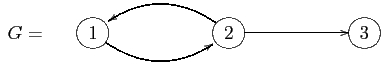
Where does such a synchronization or invariant subsystem come from? There is no apparent symmetry of $latex {\mathbb{R}}^3$ that preserves the differential equations and fixes the diagonal $latex \Delta,$ and thus could account for this invariant subsystem. It turns out that what matters is the structure of the mutual dependencies of the three subsystems making up the big system. That is, the evolution of $latex x_1$ depends only on $latex x_1$ and $latex x_2,$ the evolution of $latex x_2$ depends only on $latex x_2$ and $latex x_3,$ and the evolution of $latex x_3$ depends only on $latex x_3$ and $latex x_2.$
These dependencies can be conveniently pictured as a directed graph:
The graph $latex G$ has no symmetries. Nonetheless, the existence of the invariant subsystem living on the diagonal $latex \Delta$ can be deduced from certain properties of the graph $latex G$. The key s the existence of a surjective map of graphs
$latex \varphi :G\to G' $
from our graph $latex G$ to a graph $latex G'$ with exactly one node, call it $latex a,$ and one arrow. It is also crucial that $latex \varphi$ has the following lifting property: there is a unique way to lift the one and only arrow of $latex G'$ to an arrow of $latex G$ once we specify the target node of the lift.
We now formally define the notion of a network of regions and of a continuous-time dynamical system on such a network. Equivalently, we define a network of continuous-time dynamical systems. We start with a directed graph
$latex G=\{G_1\rightrightarrows G_0\}$
Here $latex G_1$ is the set of edges, $latex G_0$ is the set of nodes, and the two arrows assign to an edge its source and target, respectively. To each node we attach a region (more formally a manifold, possibly with corners). Here 'attach' means that we choose a function $latex {\mathcal P}:G_0 \to {\mathsf{Region}};$ it assigns to each node $latex a\in G_0$ a region $latex {\mathcal P}(a)$.
In our running example, to each node of the graph $latex G$ we attach the real line $latex {\mathbb{R}}$. (If we think of the set $latex G_0$ as a discrete category and $latex {\mathsf{Region}}$ as a category of manifolds with corners and smooth maps, then $latex {\mathcal P}$ is simply a functor.)
Thus a network of regions is a pair $latex (G,{\mathcal P})$, where $latex G$ is a directed graph and $latex {\mathcal P}$ is an assignment of regions to the nodes of $latex G.$
We think of the collection of regions $latex \{{\mathcal P}(a)\}_{a\in G_0}$ as the collection of phase spaces of the subsystems constituting the network $latex (G, {\mathcal P})$. We refer to $latex {\mathcal P}$ as a phase space function. Since the state of the network should be determined completely and uniquely by the states of its subsystems, it is reasonable to take the total phase space of the network to be the product
$latex \displaystyle{
{\mathbb{P}}(G, {\mathcal P}):= \bigsqcap_{a\in G_0} {\mathcal P}(a).
}$
In the example the total phase space of the network $latex (G,{\mathcal P})$ is $latex {\mathbb{R}}^3,$ while the phase space of the network $latex (G', {\mathcal P}')$ is the real line $latex {\mathbb{R}}$.
Finally we need to interpret the arrows. An arrow $latex b\xrightarrow{\gamma}a$ in a graph $latex G$ should encode the fact that the dynamics of the subsystem associated to the node $latex a$ depends on the states of the subsystem associated to the node $latex b.$ To make this precise requires the notion of an 'open system', or 'control system', which we define below. It also requires a way to associate an open system to the set of arrows coming into a node/vertex $latex a$.
To a first approximation an open system (or control system, I use the two terms interchangably) is a system of ODEs depending on parameters. I like to think of a control system geometrically: a control system on a phase space $latex M$ controlled by the the phase space $latex U$ is a map
$latex F: U\times M \to TM$
(here and elsewhere $latex TM$ is the tangent bundle of the space $M$) so that for all $latex (u,m)\in U\times M$, $latex F(u,m)$ is a vector tangent to $M$ at the point $m$. Given phase spaces $latex U$ and $latex M$ the set of all corresponding control systems forms a vector space which we denote by $latex\displaystyle{ \mathsf{Ctrl}(U\times M \to M}.$ (More generally one can talk about the space of control systems associated with/supported by a surjective submersion $latex Q\to M$. For us the case of the submersions of the form $latex U\times M \to M$ is general enough.)
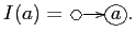
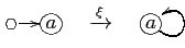
To encode the incoming arrows, we introduce the input tree $latex I(a)$ (this is a very short tree, a corolla if you like). The input tree of a node $latex a$ of a graph $latex G$ is a directed graph whose arrows are precisely the arrows of $latex G$ coming into the vertex $latex a,$ but any two parallel arrows of $latex G$ with target $latex a$ will have disjoint sources in $latex I(a)$. In the example the input tree $latex I$ of the one node of $latex a$ of $latex G'$ is the tree
There is always a map of graphs $latex \xi:I(a) \to G$. For instance for the input tree in the example we just discussed, $latex \xi$ is the map
Consequently if $latex (G,{\mathcal P})$ is a network and $latex I(a)$ is an input tree of a node of $latex G$, then $latex (I(a), {\mathcal P}\circ \xi)$ is also a network. This allows us to talk about the phase space $latex {\mathbb{P}} I(a)$ of an input tree. In our running example,
$latex {\mathbb{P}} I(a) = {\mathbb{R}}^2$
Given a network $latex (G,{\mathcal P})$, there is a vector space $latex \mathsf{Ctrl}({\mathbb{P}} I(a)\to {\mathbb{P}} a)$ of open systems associated with every node $latex a$ of $latex G$.
In our running example, the vector space associated to the one node $latex a$ of $latex (G',{\mathcal P}')$ is
$latex \mathsf{Ctrl}({\mathbb{R}}^2, {\mathbb{R}})
\simeq C^\infty({\mathbb{R}}^2, {\mathbb{R}})$
In the same example, the network $latex (G,{\mathcal P})$ has three nodes and we associate the same vector space $latex C^\infty({\mathbb{R}}^2, {\mathbb{R}})$ to each one of them.
We then construct an interconnection map
$latex \displaystyle{
{\mathcal{I}}: \bigsqcap_{a\in G_0} \mathsf{Ctrl}({\mathbb{P}} I(a)\to {\mathbb{P}} a) \to \Gamma (T{\mathbb{P}}(G, {\mathcal P})) }$
from the product of spaces of all control systems to the space of vector fields
$latex \Gamma (T{\mathbb{P}} (G, {\mathcal P}))$
on the total phase space of the network. (We use the standard notation to denote the tangent bundle of a region $latex R$ by $latex TR$ and the space of vector fields on $latex R$ by $latex \Gamma (TR)$). In our running example the interconnection map for the network $latex (G',{\mathcal P}')$ is the map
$latex \displaystyle{
{\mathcal{I}}: C^\infty({\mathbb{R}}^2, {\mathbb{R}}) \to C^\infty({\mathbb{R}}, {\mathbb{R}}), \quad f(x,u) \mapsto f(x,x).
}$
The interconnection map for the network $latex (G,{\mathcal P})$ is the map
$latex \displaystyle{
{\mathcal{I}}: C^\infty({\mathbb{R}}^2, {\mathbb{R}})^3 \to C^\infty({\mathbb{R}}^3, {\mathbb{R}}^3)}$
given by
$latex \displaystyle{
({\mathscr{I}}(f_1,f_2, f_3))\,(x_1,x_2, x_3) = (f_1(x_1,x_2), f_2(x_2,x_1),
f_3(x_3,x_2)).
}$
To summarize: a dynamical system on a network of regions is the data $latex (G, {\mathcal P}, (w_a)_{a\in G_0} )$ where $latex G=\{G_1\rightrightarrows G_0\}$ is a directed graph, $latex {\mathcal P}:{\mathcal P}:G_0\to {\mathsf{Region}}$ is a phase space function and $latex (w_a)_{a\in G_0}$ is a collection of open systems compatible with the graph and the phase space function. The corresponding vector field on the total space of the network is obtained by interconnecting the open systems.
Dynamical systems on networks can be made into the objects of a category. Carrying this out gives us a way to associate maps of dynamical systems to combinatorial data.
The first step is to form the category of networks of regions, which we call $latex {\mathsf{Graph}}/{\mathsf{Region}}.$ In this category, by definition, a morphism from a network $latex (G,{\mathcal P})$ to a network $latex (G', {\mathcal P}')$ is a map of directed graphs $latex \varphi:G\to G'$ which is compatible with the phase space functions:
$latex \displaystyle{
{\mathcal P}'\circ \varphi = {\mathcal P}.
}$
Using the universal properties of products it is easy to show that a map of networks $latex \varphi: (G,{\mathcal P})\to (G',{\mathcal P}')$ defines a map $latex {\mathbb{P}}\varphi$ of total phase spaces in the opposite direction:
$latex \displaystyle{
{\mathbb{P}} \varphi: {\mathbb{P}} G' \to {\mathbb{P}} G.
}$
In the category theory language the total phase space assignment extends to a contravariant functor
$latex \displaystyle{ {\mathbb{P}}:
{({\mathsf{Graph}}/{\mathsf{Region}})}^{\mbox{\sf {\tiny {op}}}} \to
{\mathsf{Region}}. }$
We call this functor the total phase space functor. In our running example, the map
$latex
{\mathbb{P}}\varphi:{\mathbb{R}} = {\mathbb{P}}(G',{\mathcal P}') \to
{\mathbb{R}}^3 = {\mathbb{P}} (G,{\mathcal P})$
is given by
$latex \displaystyle{
{\mathbb{P}} \varphi (x) = (x,x,x).
}$
Continuous-time dynamical systems also form a category, which we denote by $latex \mathsf{DS}$. The objects of this category are pairs consisting of a region and a vector field on the region. A morphism in this category is a smooth map of regions that intertwines the two vector fields. That is:
$latex \displaystyle{
\mathrm{Hom}_\mathsf{DS} ((M,X), (N,Y))
= \{f:M\to N \mid Df \circ X = Y\circ f\}
}$
for any pair of objects $latex (M,X), (N,Y)$ in $latex \mathsf{DS}$.
In general, morphisms in this category are difficult to determine explicitly. For example if $latex (M, X) = ((a,b), \frac{d}{dt})$ then a morphism from $latex (M,X)$ to some dynamical system $latex (N,Y)$ is simply a piece of an integral curve of the vector field $latex Y$ defined on an interval $latex (a,b)$. And if $latex (M, X) = (S^1, \frac{d}{d\theta})$ is the constant vector field on the circle then a morphism from $latex (M,X)$ to $latex (N,Y)$ is a periodic orbit of $latex Y$. Proving that a given dynamical system has a periodic orbit is usually hard.
Consequently, given a map of networks
$latex \varphi:(G,{\mathcal P})\to (G',{\mathcal P}')$
and a collection of open systems
$latex \{w'_{a'}\}_{a'\in G'_0}$
on $latex (G',{\mathcal P}')$ we expect it to be very difficult if not impossible to find a collection of open systems $latex \{w_a\}_{a\in G_0}$ so that
$latex \displaystyle{
{\mathbb{P}} \varphi: ({\mathbb{P}} G', {\mathscr{I}}' (w'))\to ({\mathbb{P}} G, {\mathscr{I}} (w))
}$
is a map of dynamical systems.
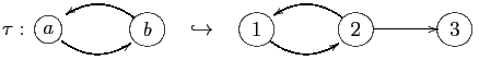
It is therefore somewhat surprising that there is a class of maps of graphs for which the above problem has an easy solution! The graph maps of this class are known by several different names. Following Boldi and Vigna we refer to them as graph fibrations. Note that despite what the name suggests, graph fibrations in general are not required to be surjective on nodes or edges. For example, the inclusion
is a graph fibration. We say that a map of networks
$latex \varphi:(G,{\mathcal P})\to (G',{\mathcal P}')$
is a fibration of networks if $latex \varphi:G\to G'$ is a graph fibration. With some work one can show that a fibration of networks induces a pullback map
$latex \displaystyle{
\varphi^*: \bigsqcap_{b\in G_0'} \mathsf{Ctrl}({\mathbb{P}} I(b)\to {\mathbb{P} b) \to
\bigsqcap_{a\in G_0} \mathsf{Ctrl}({\mathbb{P}}} I(a)\to {\mathbb{P}} a)
}$
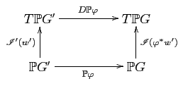
on the sets of tuples of the associated open systems. The main result of Dynamics on networks of manifolds is a proof that for a fibration of networks $latex \varphi:(G,{\mathcal P})\to (G',{\mathcal P}')$ the maps $latex \varphi^*$, $latex {\mathbb{P}} \varphi$ and the two interconnection maps $latex {\mathcal{I}}$ and $latex {\mathcal{I}}'$ are compatible:
Theorem. Let $latex \varphi:(G,{\mathcal P})\to (G',{\mathcal P}')$ be a fibration of networks of manifolds. Then the pullback map
$latex \displaystyle{ \varphi^*: \mathsf{Ctrl}(G',{\mathcal P}')\to \mathsf{Ctrl}(G,{\mathcal P})
}$
is compatible with the interconnection maps
$latex \displaystyle{
{\mathcal{I}}': \mathsf{Ctrl}(G',{\mathcal P}')) \to \Gamma (T{\mathbb{P}} G')
\quad \textrm{and} \quad
{\mathcal{I}}: (\mathsf{Ctrl}(G,{\mathcal P})) \to \Gamma (T{\mathbb{P}} G).
}$
Namely for any collection $latex w'\in \mathsf{Ctrl}(G',{\mathcal P}')$ of open systems on the network $latex (G', {\mathcal P}')$ the diagram
commutes. In other words,
$latex \displaystyle{ {\mathbb{P}} \varphi: ({\mathbb{P}}
(G',{\mathcal P}'), {\mathscr{I}}' (w'))\to ({\mathbb{P}} (G,
{\mathcal P}), {\mathscr{I}} (\varphi^* w')) }$
is a map of continuous-time dynamical systems, a morphism in $latex \mathsf{DS}$.
At this point the pure mathematician in me is quite happy: I have a theorem! Better yet, the theorem solves the puzzle at the beginning of this post. But if you have read this far, you may well be wondering: "ok, you told us about your theorem. Very nice. Now what?"
There is plenty to do. On the practical side of things, the continuous-time dynamical systems are much too limited for contemporary engineers. Most of the engineers I know care a lot more about hybrid systems. These kinds of systems exhibit both continuous time behavior and abrupt transitions, hence the name. For example, anti-lock breaks on a car is just that kind of a system — if a sensor detects that the car is skidding and the foot break is pressed, it starts pulsing the breaks. This is not your father's continuous time dynamical system. Hybrid dynamical systems are very hard to understand. They have been all the rage in the engineering literature for the last 10-15 years. Saddly most pure mathematicians never heard of them. It would be intersting to extend the theorem I am bragging about to hybrid systems.
Here is another problem that may be worth thinking about: how much of the theorem holds up to numerical simulation? My feeling is that any explicit numerical integration method will behave well. Implicit methods I am not sure about.
And finally a more general issue. John has been talking about networks quite a bit on this blog. But his networks and my networks look like very different mathematical structures. What do they have in common besides nodes and arrows?
What mathematical structure are they glimpses of?