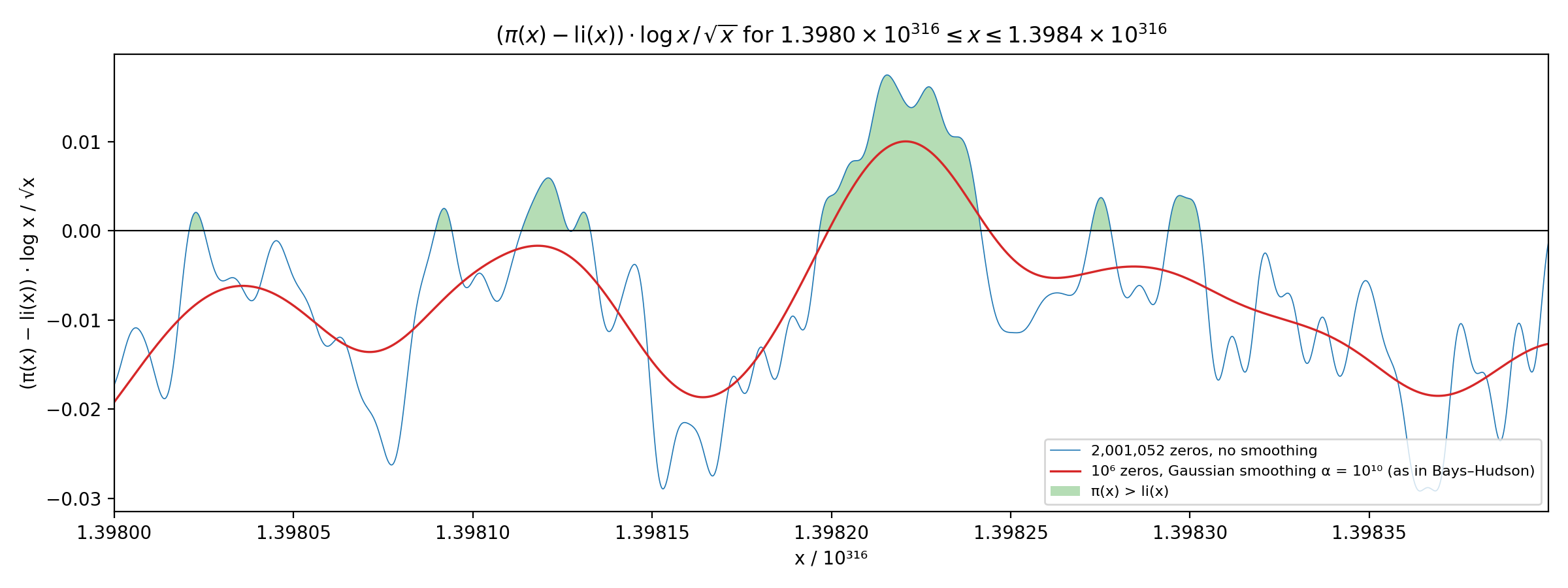
These graphs show \(\pi(x) - \mathrm{li}(x)\) near one of first places it is known to become positive: \(x \approx 1.39822 \times 10^{316}\). Here \(\pi(x)\) is the number of primes \(\le x\), while \[ \mathrm{li}(x) = \int_0^x \frac{ds}{\log s} \] is a function called the logarithmic integral.
For all \(x\) where \(\pi(x)\) can actually be counted, \(\pi(x) < \mathrm{li}(x)\). Littlewood proved in 1914 that the difference nonetheless changes sign infinitely often. Later Skewes gave an explicit upper bound for the first sign change: \[ e^{e^{e^{e^{7.705}}}} \approx 10^{10^{10^{964}}} \] This is famously enormous number sometimes called Skewes' number, often said to be the largest number used in a serious piece of mathematics---not just bigness for the sake of bigness. Lehman (1966) found a method that brought the bound down to about \(1.65 \times 10^{1165}\), and te Riele (1987) lowered it to about \(6.66 \times 10^{370}\).
In a heroic piece of work, Bays and Hudson (2000) then proved that there are at least \(10^{153}\) integers \(x\) near \(1.39822 \times 10^{316}\) with \(\pi(x) > \mathrm{li}(x)\). Their paper includes many graphs, but their printed figures are of poor quality. I've always been curious how they did what they did, and I think the world deserves better pictures of this amazing result, so I have redone a bit of their work here. My calculations use twice as many zeros of the Riemann zeta function as they had access to, and the computation now takes a couple of seconds on a laptop. Here is my version of their Figure 2b:
Bays and Hudson's proof does not depend on the Riemann hypothesis, and neither do the later proofs mentioned below. Their graphs are another matter—and the same is true for the graphs here. It's hard to get a really precise approximation to \(\pi(x)\) for huge numbers \(x\) without using the Riemann hypothesis, since our best formula for it is a sum over zeros of the Riemann zeta function, and even a single zero off the critical line \(z = \frac{1}{2}\) could have a big effect. However, a smoothed version of \(\pi(x)\) is much less sensitive to this problem.
The red curves in my graphs are smoothed, and since even it goes above zero for a long stretches, Bays and Hudson were able to prove that \(\pi(x) > \mathrm{li}(x)\) for some \(x\) near \(1.39822 \times 10^{316}\). On the other hand, the blue curve is not deliberately smoothed. Its calculation assumes the Riemann hypothesis, and could change substantially if that was wrong! There could also be other problems, as I'll explain. But it's probably very close to correct if the Riemann hypothesis holds.
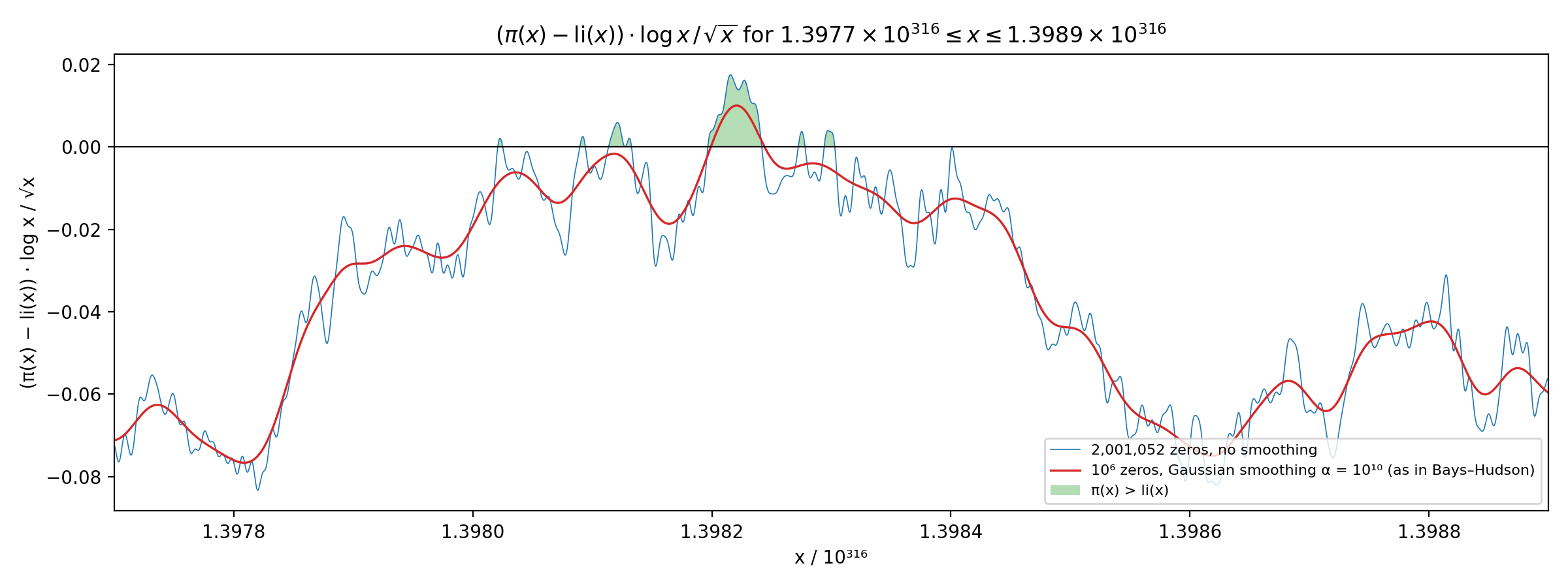
Intriguingly, \(\pi(x) - \mathrm{li}(x)\) also becomes positive for some slightly smaller numbers, in a region around \(1.39717 \times 10^{316}\). Patrick Demichel spotted this region, Saouter and Demichel proved it exists in 2010, and Saouter, Trudgian and Demichel pinned it down more sharply in 2015. Here is a wider view that also includes the sharp spike around \(1.39717 \times 10^{316}\).
Nobody can compute \(\pi(x)\) exactly for numbers so large as \(10^{316}\). What we can compute is an approximation coming from Riemann's explicit formula, which expresses \(\pi(x) - \mathrm{li}(x)\) as a sum over the nontrivial zeros \(\rho = \tfrac12 + i\gamma\) of the zeta function. Assuming the Riemann hypothesis, write \(u = \log x\) and measure \(\pi(x) - \mathrm{li}(x)\) in units of \(\sqrt{x} / \log x\):
\[ D(u) = \bigl(\pi(x) - \mathrm{li}(x)\bigr)\,\frac{\log x}{\sqrt{x}} \;\approx\; -\Bigl(1 + \frac{2}{u} + \frac{8}{u^2}\Bigr) \;-\; 2\sum_{0<\gamma\le T} \mathrm{Re}\!\left[\frac{e^{i\gamma u}}{\rho}\Bigl(1 + \frac{1}{\rho u}\Bigr)\right] \]The symbol \(\approx\) hides several approximations of quite different kinds; the section What is rigorous and what is not explains exactly what it means. The term
\[ −(1 + 2/u + 8/u²) \]comes from the squares of primes: \(\pi(x)\) counts primes, but the explicit formula naturally counts prime powers, and correcting for squares costs about \(\tfrac12 \mathrm{li}(\sqrt{x})\). (Higher powers contribute much less.)
This term is why \(\pi(x) - \mathrm{li}(x)\) is usually negative, by about \(\sqrt{x} / \log x\). More interesting is the sum over zeros: each zero contributes an oscillation in \(\log x\) with frequency \(\gamma\) and amplitude roughly \(1/\gamma\). \(D(u)\) becomes positive, and \(\pi(x) - \mathrm{li}(x)\) with it, only when many low zeros happen to oscillate in phase strongly enough to overcome the \(-1\).
On the graphs, \(D > 0\) means \(\pi(x) > \mathrm{li}(x)\), and the vertical axis is in units of \(\sqrt{x} / \log x\), which is about \(10^{155}\) near \(x = 10^{316}\).
Each graph shows two curves:
The zeros come from Andrew Odlyzko's table zeros6: the first 2,001,052 zeros, accurate to within \(4 \times 10^{-9}\). Bays and Hudson needed a personal favor from Odlyzko to get a million zeros. Today the same table is a free download, and it is even packaged on PyPI as passagemath-database-odlyzko-zeta. As a check, a few of the values (zeros number 1, 1000, 500,000, \(10^6\) and \(2 \times 10^6\)) were compared against certified computations from the Arb library. They agree to better than \(10^{-9}\).
Each point on a curve is a sum of a million or two sine waves. Summing directly at 8000 points would take about \(10^{10}\) operations. Instead the program uses a nonuniform fast Fourier transform (the FINUFFT library), which finishes in about a second on one core. Two precautions matter: the program never forms \(x\) itself, only \(u = \log x\), and it computes each phase \(\gamma u\) modulo \(2\pi\) carefully, because \(\gamma u\) reaches about \(10^9\).
Narrow window, \(1.3977\)–\(1.3989 \times 10^{316}\). This graph shows our estimate of \((\pi(x) - \mathrm{li}(x)) \cdot \log x / \sqrt{x}\) for \(x\) between \(1.3977 \times 10^{316}\) and \(1.3989 \times 10^{316}\).
This is the same range as Figure 2b in Bays and Hudson's paper. The region they proved positive is the green hump near \(1.39822 \times 10^{316}\). \(D\) usually hovers around \(-1\), but throughout this window the low zeros happen to be nearly in phase, lifting it close to zero. Even so it is a narrow escape: the blue curve rises only about 0.017 above zero. The red curve peaks at about \(+0.010\), which is what lets Lehman's theorem prove that \(\pi(x) > \mathrm{li}(x)\) somewhere in this region. Two smaller bumps of the blue curve, near 1.3981 and 1.3983, barely cross zero; they are about as big as the truncation error, so they could be artifacts.
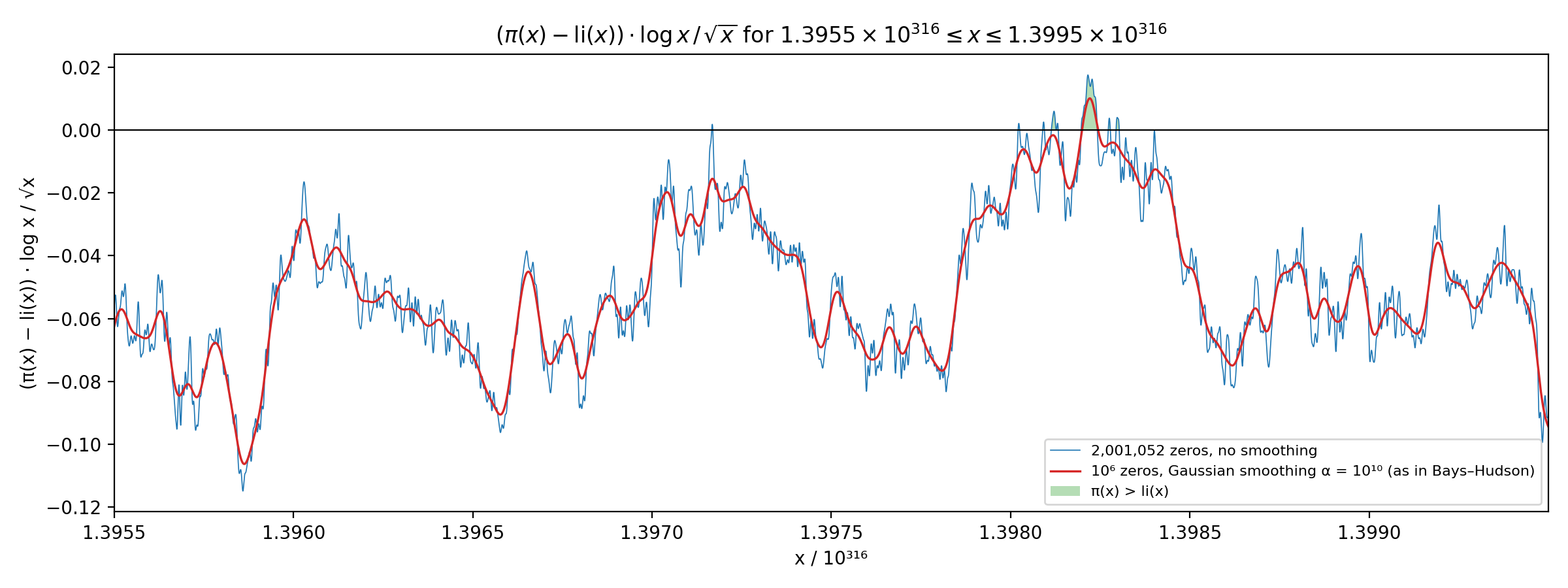
Wider view, \(1.3955\)–\(1.3995 \times 10^{316}\). This zooms out to show what lies just to the left.
The thin spike at about \(1.39717 \times 10^{316}\) is a second positive region, found after Bays and Hudson. Saouter and Demichel proved \(\pi(x) > \mathrm{li}(x)\) there in 2010, and Saouter, Trudgian and Demichel later narrowed it to an interval centred at \(\log x = 727.951335426\). In this graph the blue curve rises only about 0.0018 above zero at that spike. That is no larger than the error from using only two million zeros, so this graph alone could not prove the spike is positive. The proof used about \(5 \times 10^8\) zeros. The red curve, smoothed too heavily to see so narrow a spike, stays below zero there.
The red curve could be given rigorous error bars; the blue curve cannot; and \(\pi(x) - \mathrm{li}(x)\) itself, point by point, is out of reach near \(10^{316}\).
Where the formula comes from. The starting point is Riemann's explicit formula for his prime-power counting function \(J(x) = \sum_{p^k \le x} 1/k\). For \(x > 1\) it says
\[ J(x) = \mathrm{li}(x) - \sum_\rho \mathrm{li}(x^\rho) - \log 2 + \int_x^\infty \frac{dt}{t(t^2-1)\log t}, \]where the sum over zeros converges only conditionally and must be taken in order of increasing \(|\gamma|\). Proofs are in the books of Edwards and Ingham. Möbius inversion gives \(\pi(x) = \sum_n \mu(n) J(x^{1/n})/n\), so
\[ \pi(x) - \mathrm{li}(x) = -\tfrac12 \mathrm{li}(\sqrt{x}) - \sum_\rho \mathrm{li}(x^\rho) + (\text{smaller terms}). \]Expanding \(\mathrm{li}(\sqrt{x}) = (2\sqrt{x}/u)(1 + 2/u + 8/u^2 + \cdots)\) and \(\mathrm{li}(x^\rho) = \mathrm{Ei}(\rho u) = (x^\rho/(\rho u))(1 + 1/(\rho u) + \cdots)\), multiplying by \(u/\sqrt{x}\), and pairing each zero with its complex conjugate gives the formula for \(D(u)\). Apart from the \(1/(\rho u)\) correction and the Gaussian damping, this is the function \(g(x)\) in Table 1 of Bays and Hudson.
What the \(\approx\) means. Three separate approximations are involved, and they are very different in character.
What the \(\pm 0.002\) means. Assuming the Riemann hypothesis, \(D(u)\) is an almost periodic function of \(u\), which is the setting Rubinstein and Sarnak use. A Parseval identity for such functions should then give the long-run mean square of the omitted tail as about \(\sum_{\gamma > T} 2/|\rho|^2 \approx (0.002)^2\). That is a statement about averages over very long stretches of \(u\). It does not bound the error at any particular point, or even across our window. Reading \(\pm 0.002\) as the typical error at each point of the blue curve amounts to treating the omitted terms as random noise. That is a heuristic, though the check at \(x = 10^{20}\) is consistent with it. So the blue curve is a good picture, not a proof.
The smoothed curve. Every positive region found so far was proved using a theorem of Lehman (1966), stated as Theorem 1 in Bays and Hudson's paper. Instead of trying to pin down \(\pi(x) - \mathrm{li}(x)\) at a single point, Lehman's theorem handles a weighted average of it: the average of \(D(u)\) against a Gaussian bump of width \(1/\sqrt{\alpha}\) centred at some point \(\omega\). The theorem says this average equals \(-1\) minus a sum over the zeros, with each zero damped by a factor \(e^{-\gamma^2/2\alpha}\), plus an error term with explicit bounds that hold for every \(\omega\). The red curve is essentially this damped sum, plotted as a function of \(\omega\). The key point is that an average can only be positive if the function being averaged is positive somewhere. So if the damped sum is above zero by more than the largest possible error at some \(\omega\), then \(\pi(x) > \mathrm{li}(x)\) for some \(x\) with \(\log x\) near \(\omega\). Bays and Hudson proved their result this way, and later authors used refined versions of the same theorem.
The smoothing is what gives this approach its teeth. The damping makes the contribution of the omitted zeros decay like \(e^{-T^2/2\alpha}\), so stopping at height \(T\) costs almost nothing. With these parameters the total error is a few thousandths, dominated by a prime-power term of size about \(2/\omega\) to \(3/\omega\), where \(\omega \approx 728\). So one could draw an upper and a lower curve that provably bracket the smoothed function. Wherever the lower curve is above zero, \(\pi(x) > \mathrm{li}(x)\) somewhere nearby.
This holds without assuming the Riemann hypothesis. Lehman's theorem needs the Riemann hypothesis only up to a finite height, which has been verified: Platt and Trudgian have now checked it up to height \(3 \times 10^{12}\). Any hypothetical zeros off the critical line beyond that height are covered by an extra error term, which the Gaussian smoothing makes harmless. For Bays and Hudson's parameters this term is smaller than \(10^{-2001}\). So the positive regions near \(1.39822 \times 10^{316}\) and \(1.39717 \times 10^{316}\) are established unconditionally.
The method is one-sided, though. It can prove that crossings exist, but a negative average says nothing about a narrow positive spike hiding inside it.
Earlier crossings. Bays and Hudson observe (p. 1287) that current knowledge cannot rule out sign changes of \(\pi(x) - \mathrm{li}(x)\) over gaps as large as \(10^{300}\) near \(10^{316}\). For the same reason, nobody can currently rule out a crossing somewhere below \(1.397 \times 10^{316}\). Bays and Hudson thought none is likely. Their Figure 1 marks near-misses around \(10^{176}\), \(10^{179}\), \(10^{190}\), \(10^{260}\) and \(10^{298}\). Rigorously, it is known only that \(\pi(x) < \mathrm{li}(x)\) for all \(x \le 10^{19}\), as Revers (2025) notes. So between \(10^{19}\) and about \(1.397 \times 10^{316}\) the question remains open!
The graphs were made with a short Python program, skewes_window.py, using NumPy, mpmath, Matplotlib and FINUFFT.
The main papers
The explicit formula and its approximations
Historical background
Data and software