

|
|
|
|
In our quest to understand the true nature of random permutations, Part 7 took us into a deeper stratum: their connection to Poisson distributions. I listed a few surprising facts. For example, these are the same:
Here the raindrops are Poisson distributed, and 'huge' means I'm taking a limit as the size of a finite set goes to infinity.
Now let's start trying to understand what's going on here! Today we'll establish the above connection between raindrops and random permutations by solving this puzzle:
Puzzle 12. If we treat the number of cycles of length \(k\) in a random permutation of an \(n\)-element set as a random variable, what do the moments of this random variable approach as \(n \to \infty\)?
First, let me take a moment to explain moments.
To be a bit more formal about our use of probability theory: I'm treating the symmetric group \(S_n\) as a probability measure space where each permutation has measure \(1/n!\). Thus, any function \(f \colon S_n \to \mathbb{R}\) can be thought of as a random variable.
One thing we do with this random variable is compute its expected value or mean, defined by
\[ E(f) = \frac{1}{n!} \sum_{\sigma \in S_n} f(\sigma) \]But this only says a little about our random variable. To go further, we can compute \(E(f^p)\) for any natural number \(p\). This is called the \(p\)th moment of \(f\).
If the mean of \(f\) is zero, its second moment \(E(f^2)\) is called its variance: it's a measure of how spread-out our random variable is. If the mean of \(f\) is zero, its third moment \(E(f^3)\) is a measure of how 'skewed' our random variable is:
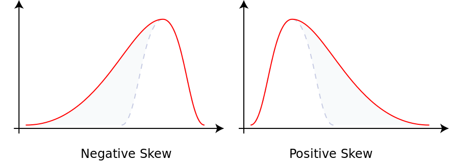
Suitably normalized, \(E(f^3)\) gives a quantity called the 'skewness'. And if the mean of \(f\) is zero, its fourth moment \(E(f^4)\) is a measure of how 'long-tailed' our random variable is, beyond what you'd expect from its variance.. Suitably normalized, \(E(f^4)\) gives a quantity called the 'kurtosis'. This sounds like a disease, but it's from a Greek word that means 'arching'.
I don't know if there are names for the higher moments. Somebody must have thought of some, and after 'skewness' and 'kurtosis' I'd expect terms like 'anomie', 'dyspepsia' and 'lassitude', but whatever they are, they haven't caught on.
While the higher moments say increasingly subtle things about our random variable, taken together they tell us everything we'd want to know about it, at least in good cases.
I will resist expanding on this, because I want to start solving the puzzle!
For this, we're interested in the number of cycles of length \(k\) in a permutation. This defines a function
\[C_k \colon S_n \to \mathbb{N} \]which we can treat as a random variable. What are its moments? In Puzzle 7 we saw that its mean is \(1/k\) whenever \(n \ge k\). Of course it's zero when \(n \lt k\), since in this case a cycle of length \(k\) is too big to be possible. So, we have
\[ E(C_k) = \left\{ \begin{array}{ccl} 1/k & \mathrm{if} & k \lt n \\ \\ 0 & \mathrm{if} & k \ge n \end{array} \right. \]What about the second moment, \(E(C_k^2)\)? This is the expected number of ordered pairs of cycles of length \(k\).
It's actually easier to compute \(E(C_k(C_k - 1))\). This is the expected number of ordered pairs of distinct cycles of length \(k\). Equivalently, it's the expected the number of ordered pairs of disjoint cycles of length \(k\).
Why does this help?
Here's why. Instead of going through all permutations and counting pairs of disjoint cycles of length \(k\), we can reverse the order: go through pairs of disjoint subsets of size \(k\) and counting permutations having these as cycles! Since all pairs of disjoint subsets of size \(k\) 'look alike', this is easy.
So, to compute \(E(C_k(C_k - 1))\), we count the pairs of disjoint \(k\)-element subsets \(S_1, S_2\) of our \(n\)-element set. For any such pair we count the permutations having \(S_1\) and \(S_2\) as cycles. We multiply these numbers, and then we divide by \(n!\).
If \(2k \gt n\) the answer is obviously zero. Otherwise, there are
\[ \binom{n}{k, k, n-2k} = \frac{n!}{k! \, k! \, (n-2k)!} \]ways to choose \(S_1\) and \(S_2\) — this number is called a multinomial coefficient. For each choice of \(S_1, S_2\) there are \((k-1)!^2\) ways to make these sets into cycles and \((n-2k)!\) ways to pick a permutation on the rest of our \(n\)-element set. Multiplying these numbers we get
\[ (k-1)!^2 \, (n-2k)! \, \frac{n!}{k! \, k! \, (n-2k)!} = \frac{n!}{k^2} \]Dividing by \(n!\) we get our answer:
\[ E(C_k(C_k - 1)) = \frac{1}{k^2} \]It would be nice to explain why the answer is so much simpler than the calculation. But let's move on to higher moments!
Computing \(E(C_k(C_k-1)\) was just as good as computing \(E(C_k^2)\), since we already knew \(E(C_k)\). Continuing on with this philosophy, let's compute the expected value of the \(p\)th falling power of \(C_k\), which is defined by
\[ C_k^{\underline{p}} = C_k (C_k - 1) \, \cdots \, (C_k - p + 1) \]This random variable counts the ordered \(p\)-tuples of disjoint cycles of length \(k\).
Last time I explained how to express ordinary powers in terms of falling powers, so we can compute the moments \(E(C_k^p)\) if we know the expected values \(E(C_k^{\underline{p}})\). This trick is so popular that these expected values \(E(C_k^{\underline{p}})\) have a name: they're called factorial moments. I'd prefer to call them 'falling moments', but I'm not king of the world... yet.
To compute \(E(C_k^{\underline{p}})\), we just generalize what I did a moment ago.
First we count the \(p\)-tuples of disjoint \(k\)-element subsets \(S_1, \dots, S_p\) of our \(n\)-element set. For any such \(p\)-tuple we count the permutations having these sets \(S_1, \cdots, S_p\) as cycles. We multiply these numbers, and then we divide by \(n!\).
If \(pk \gt n\) the answer is zero. Otherwise, there are
\[ \binom{n}{k, k, \dots, k, n-pk} = \frac{n!}{k!^p (n-pk)!} \]ways to choose a \(p\)-tuple of disjoint \(k\)-element subsets. There are \((k-1)!^p\) ways to make these sets into cycles and \((n-p k)!\) ways to pick a permutation on the rest of our \(n\)-element set. Multiplying all these, we get
\[ (k-1)!^p \, (n-p k)! \, \frac{n!}{k!^p \, (n-p k)!} = \frac{n!}{k^p} \]Dividing this by \(n!\) we get our answer:
\[ E(C_k^{\underline{p}}) = \frac{1}{k^p} \]Again, lots of magical cancellations! Summarizing everything so far, we have
\[ E(C_k^{\underline{p}}) = \left\{ \begin{array}{ccl} \displaystyle{\frac{1}{k^p}} & \mathrm{if} & p k \le n \\ \\ 0 & \mathrm{if} & p k \gt n \end{array} \right. \]Now, last time we saw that the factorial moments of a Poisson distribution with mean \(1\) are all equal to \(1\). The same sort of calculation shows that the \(p\)th factorial moment of a Poisson distribution with mean \(1/k\) is \(1/k^p\).
So, we're seeing that the first \(\lfloor n/k \rfloor\) factorial moments of the random variable \(C_k\) match those of a Poisson distribution with mean \(1/k\). But we can express ordinary powers in terms of falling powers. I showed how this works in Part 8:
\[ x^p = \sum_{i = 0}^p \left\{ \begin{array}{c} p \\ i \end{array} \right\} \; x^{\underline{i}} \]Even if you don't understand the coefficients, which are Stirling numbers of the second kind, it follows straightaway that we can express the first \(\lfloor n/k \rfloor\) moments of a random variable in terms of its first \(\lfloor n/k \rfloor\) factorial moments.
So, the first \(\lfloor n/k\ \rfloor\) moments of \(C_k\) match those of the Poisson distribution with mean \(1/k\).
This solves the puzzle! Of course there are various notions of convergence, but now is the not the time for subtleties of analysis. If we fix a value of \(p\), we know now that the \(p\)th moment of \(C_k\) approaches that of the Poisson distribution with mean \(1/k\) as \(n \to \infty\).
And if we can get the analysis to work out, it follows that these are equal:
One thing I need to do is next is examine the computations that led to this result and figure out what they mean. Last time we worked out the factorial moments of a Poisson distribution. This time we worked out the factorial moments of the random variable that counts cycles of length \(k\). The combinatorics involved in why these calculations match as well as they do — that's what I need to ponder. There is something nice hiding in here. If you want to help me find it, that'd be great!
Roland Speicher has already pointed me to a good clue, which I need to follow up on.
By the way, if you think my answer to the puzzle was not sufficiently concrete, I can rewrite it a bit. Last time we saw that the \(p\)th moment of the Poisson distribution with mean \(1\) is the number of partitions of a \(p\)-element set, also called the Bell number \(B_p\). The \(p\)th moment of the Poisson distribution with mean \(1/k\) is thus \(B_p/k^p\).
So, for any \(p\), we have
\[ \lim_{n \to \infty} E(C_k^p) = \frac{B_p}{k^p} \]You can also read comments on the n-Category Café, and make your own comments or ask questions there!
|
|
|
|