

|
|
|
|
Last time I promised to show you how the problem of a little ball rolling on a big stationary ball can be described using an 8-dimensional number system called the split octonions... if the big ball has a radius that.s 3 times the radius of the little one!
So, let's get started.

First, I must admit that I lied.
Lying is an important pedagogical technique. The teacher simplifies the situation, so the student doesn't get distracted by technicalities. Then later—and this is crucial!—the teacher admits that certain statements weren't really true, and corrects them. It always makes me uncomfortable to do this. But it works better than dumping all the technical details on the students right away. In classes, I sometimes deal with my discomfort by telling the students: "Okay, now I'm going to lie a bit..."
What was my lie? Instead of an ordinary ball rolling on another ordinary ball, we need a 'spinorial' ball rolling on a 'projective' ball.
Let me explain that.
In physics, a spinor is a kind of particle that you need to turn around twice before it comes back to the way it was. Examples include electrons and protons.
If you give one of these particles a full 360° turn, which you can do using a magnetic field, it changes in a very subtle way. You can only detect this change using clever tricks. For example, take a polarized beam of electrons and send it through a barrier with two slits cut out. Each electron goes through both slits, because it's a wave as well as a particle. Next, put a magnetic field next to one slit that's precisely strong enough to rotate the electron by 360° if it goes through that slit. Then, make the beams recombine, and see how likely it is for electrons to be found at different locations. You'll get different results than if you turn off the magnetic field that rotates the electron!
However, if you rotate a spinor by 720°—that is, two full turns—it comes back to exactly the way it was.
This may seem very odd, but when you understand the math of spinors you see it all makes sense. It's a great example of how you have to follow the math where it leads you. If something is mathematically allowed, nature may take advantage of that possibility, regardless of whether it seems odd to you.
So, I hope you can imagine a 'spinorial' ball, which changes subtly when you turn it 360° around any axis, but comes back to its original orientation when you turn it around 720°. If you can't, I'll present the math more rigorously later on. That may or may not help.
What's a 'projective' ball? It's a ball whose surface is not a sphere, but a projective plane. A projective plane is a sphere that's been modified so that diametrically opposite points count as the same point. The north pole is the same as the south pole, and so on!
In geography, the point diametrically opposite to some point on the Earth's surface is called its antipodes, so let's use that term. There's a website that lets you find the antipodes of any place on Earth. Unfortunately the antipodes of most famous places are under water! But the antipodes of Madrid is in New Zealand, near Wellington:

When we roll a little ball on a big 'projective' ball, when the little ball reaches the antipodes of where it started, it counts as being back to its original location.
If you find this hard to visualize, imagine rolling two indistinguishable little balls on the big ball, that are always diametrically opposite each other. When one little ball rolls to the antipodes of where it started, the other one has taken its place, and the situation looks just like when you started!
Now let's combine these ideas. Imagine a little spinorial ball rolling on a big projective ball. You need to turn the spinorial ball around twice to make it come back to its original orientation. But you only need to roll it halfway around the projective ball for it to come back to its original location.
These effects compensate for each other to some extent. The first makes it twice as hard to get back to where you started. The second makes it twice as easy!
But something really great happens when the big ball is 3 times as big as the little one. And that's what I want you to understand.
For starters, consider an ordinary ball rolling on another ordinary ball that's the same size. How many times does the rolling ball turn as it makes a round trip around the stationary one? If you watch this you can see the answer:
Follow the line drawn on the little ball. It turns around not once, but twice!
Next, consider one ball rolling on another whose radius is 2 times as big. How many times does the rolling ball turn as it makes a round trip?
It turns around 3 times.
And this pattern continues! I don't have animations proving it, so either take my word for it, read our paper, or show it yourself.
In particular, a ball rolling on a ball whose radius is 3 times as big will turn 4 times as it makes a round trip. So, by the time the little ball rolls halfway around the big one, it will have turned around twice!
But now suppose it's a spinorial ball rolling on a projective plane. This is perfect. Now when the little ball goes halfway around big ball, it returns to its original location! And turning around the little ball twice gets it back to its original orientation!
So, there is something very neat about a spinorial ball rolling on a projective ball whose radius is exactly 3 times as big. And this is just the start. Now the split octonions get involved!
The key is to ponder a curious sort of geometry, which I'll call the rolling ball geometry. This has 'points' and 'lines' which are defined in a funny way.
A point is any way a little spinorial ball can touch a projective ball that is 3 times as big. The lines are certain sets of points. A line consists of all the points we reach as the little ball rolls along some great circle on the big one, without slipping or twisting.
Of course these aren't 'points' and 'lines' in the usual sense. But ever since the late 1800s, when mathematicians got excited about projective geometry—which is the geometry of the projective plane—we've enjoyed studying all sorts of strange variations on Euclidean geometry, with weirdly defined 'points' and 'lines'. The rolling ball geometry fits very nicely into this tradition.
But the amazing thing is that we can describe points and lines of the rolling ball geometry in a completely different way, using the split octonions.
How does it work? As I said last time, the split octonions are an 8-dimensional number system. We build them as follows. We start with the ordinary real numbers. Then we throw in 3 square roots of -1, called $latex i, j,$ and $latex k$, obeying
$$ ij = -ji = k$$ $$ jk = -kj = i$$ $$ ki = -ik = j$$
At this point we have a famous 4-dimensional number system called the quaternions. Quaternions are numbers like
$$ a + bi + cj + dk $$
where \( a,b,c,d\) are real numbers and \( i, j, k\) are the square roots of -1 we just created.
To build the octonions, we would now throw in another square root of -1. But to build the split octonions, we instead throw in a square root of +1. Let's call it \( \ell\). The hard part is saying what rules it obeys when we start multiplying it with other numbers in our system.
For starters, we get three more numbers \( \ell i, \ell j, \ell k\). We decree these to be square roots of +1. But what happens when we multiply these with other things? For example, what is \( \ell i \) times \( j\), and so on?
Since I don't want to bore you, I'll just get this over with quickly by showing you the multiplication table:
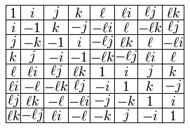
This says that \( \ell i\) (read down) times \( j \) (read across) is \( -\ell k\), and so on.
Of course, this table is completely indigestible. I could never remember it, and you shouldn't try. This is not the good way to explain how to multiply split octonions! It's the lazy way. To really work with the split octonions you need a more conceptual approach, which John Huerta and I explain in our paper. But this is just a quick tour... so, on with the tour!
A split octonion is any number like
$$ a + bi + cj + dk + e \ell + f \ell i + g \ell j + h \ell k$$
where $latex a,b,c,d,e,f,g,h$ are real numbers. Since it takes 8 real numbers to specify a split octonion, we say they're an 8-dimensional number system. But to describe the rolling ball geometry, we only need the imaginary split octonions, which are numbers like
$$ x = bi + cj + dk + e \ell + f \ell i + g \ell j + h \ell k $$
The imaginary split octonions are 7-dimensional. 3 dimensions come from square roots of -1, while 4 come from square roots of 1.
We can use them to make up a far-out variant of special relativity: a universe with 3 time dimensions and 4 space dimensions! To do this, define the length of an imaginary split octonion \(x\) to be the number \( \|x \| \) with
$$ \|x\|^2 = -b^2 - c^2 - d^2 + e^2 + f^2 + g^2 + h^2 $$
This is a mutant version of the Pythagorean formula. The length \(\|x\|\) is real, in fact positive, for split octonions that point in the space directions. But it's imaginary for those that point in the time directions!
This should not sound weird if you know special relativity. In special relativity we have spacelike vectors, whose length squared is positive, and timelike ones, whose length squared is negative.
If you don't know special relativity—well, now you see how revolutionary Einstein's ideas really are.
We also have vectors whose length squared is zero! These are called null. They're also called lightlike, because light rays point along null vectors. In other words: light moves just as far in the space directions as it does in the time direction, so it's poised at the brink between being spacelike and timelike.
I'm sure you're wondering where all this is going. Luckily, we're there. We can describe the rolling ball geometry using the imaginary split octonions! Let me state it and then chat about it:
Theorem. There is a one-to-one correspondence between points in the rolling ball geometry and light rays through the point 0 in the imaginary split octonions. Under this correspondence, lines in the rolling ball geometry correspond to planes containing the point 0 in the imaginary split octonions with the property that whenever \( x \) and \( y \) lie in this plane, then \( xy = 0.\)
Even if you don't get this, you can see it's describing the rolling ball geometry in terms of stuff about the split octonions. An immediate consequence is that any symmetry of the split octonions is a symmetry of the rolling ball geometry.
The symmetries of the split octonions form a group called 'the split form of G2'. With more work, we can show the converse: any symmetry of the rolling ball geometry is a symmetry of the split octonions. So, the symmetry group of the rolling ball geometry is precisely the split form of G2.
So what?
Well, G2 is an 'exceptional group'—one of five groups that were discovered only when mathematicians like Killing and Cartan systematically started trying to classify groups in the late 1800s. The exceptional groups didn't fit in the lists of groups mathematicians already knew.
If, as Tim Gowers has argued, some math is invented while some is discovered, the exceptional groups were discovered. Finding them was like going to the bottom of the ocean and finding weird creatures you never expected. These groups were—and are—hard to understand! They have dry, technical sounding names: E6, E7, E8, F4, and G2. They're important in string theory—but again, just because the structure of mathematics forces it, not because people wanted it.
The exceptional groups can all be described using the octonions, or split octonions. But the octonions are also rather hard to understand. The rolling ball geometry, on the other hand, is rather simple and easy to visualize. So, it's a way of bringing some exotic mathematics a bit closer to ordinary life.
Well, okay—in ordinary life you'd probably never thought about a spinorial ball rolling on a projective ball. But still: spinors and projective planes are far less exotic than split octonions and exceptional Lie groups. Any mathematician worth their salt knows about spinors and projective planes. They're things that make plenty of sense.
I think now is a good time for most of you nonmathematicians to stop reading. I'll leave off with a New Year's puzzle:
Puzzle: Relative to the fixed stars, how many times does the Earth turn around its axis in a year?
Bye! It was nice seeing you!
Still here? Cool. I want to wrap up by presenting the theorem in a more precise way, and then telling the detailed history of the rolling ball problem.
How can we specify a point in the rolling ball geometry? We need to say the location where the little ball touches the big ball, and we need to describe the 'orientation' of the little ball: that is, how it's been rotated.
The point where the little ball touches the big one is just any point on the surface of the big ball. If the big ball were an ordinary ball this would be a point on the sphere, \( S^2\). But since it's a projective ball, we need a point on the projective plane, \( \mathbb{R}\mathrm{P}^2\).
To describe the orientation of the little ball we need to say how it's been rotated from some standard orientation. If the little ball were an ordinary ball we'd need to give an element of the rotation group, \( \mathrm{SO}(3).\) But since it's a spinorial ball we need an element of the double cover of the rotation group, namely the special unitary group \( \mathrm{SU}(2).\)
So, the space of points in the rolling ball geometry is
$$X = \mathbb{R}\mathrm{P}^2 \times \mathrm{SU}(2)$$
This makes it easy to see how the imaginary split octonions get into the game. For starters, \( \mathrm{SU}(2)\) is isomorphic to the group of unit quaternions. We can define the absolute values of quaternions in a way that copies the usual formula for complex numbers:
$$\displaystyle{ |a + bi + cj + dk| = \sqrt{a^2 + b^2 + c^2 + d^2} } $$
The great thing about the quaternions is that if we multiply two of them, their absolute values multiply. In other words, if \( q\) and \( q'\) are two quaternions,
$$|qq'| = |q| |q'| $$
This implies that the quaternions with absolute value 1—the unit quaternions—are closed under multiplication. In fact, they form a group. And in fact, this group is just SU(2) in mild disguise!
The unit quaternions form a sphere. Not an ordinary '2-sphere' of the sort we've been talking about so far, but a '3-sphere' in the 4-dimensional space of quaternions. We call that \( S^3.\)
So, the space of points in the rolling ball is isomorphic to a projective plane times a 3-sphere:
$$X \cong \mathbb{R}\mathrm{P}^2 \times S^3 $$
But since the projective plane \( \mathbb{R}\mathrm{P}^2\) is the sphere \( S^2\) with antipodal points counted as the same point, our space of points is
$$\displaystyle{ X \cong \frac{S^2 \times S^3}{(p,q) \sim (-p,q)}} $$
Here dividing or 'modding out' by that stuff on the bottom says that we count any point \( (p,q)\) in \( S^2 \times S^3\) as the same as \( (-p,q).\)
The cool part is that while \( S^3\) is the unit quaternions, we can think of \( S^2\) as the unit imaginary quaternions, where an imaginary quaternion is a number like
$$bi + cj + dk $$
So, we're describing a point in the rolling ball geometry using a unit quaternion and a unit imaginary quaternion. That's cool. But we can improve this description a bit using a nonobvious fact:
$$\displaystyle{ X \cong \frac{S^2 \times S^3}{(p,q) \sim (-p,-q)}} $$
There's an extra minus sign here! Now we're counting any point \( (p,q)\) in \( S^2 \times S^3\) as the same as \( (-p,-q).\) In Proposition 2 of our paper we give an explicit formula for this isomorphism, which is important.
But never mind. Here's the point of this improvement: we can now describe a point in the rolling ball geometry as a light ray through the origin in the imaginary split octonions! After all, any split octonion is of the form
$$ a + bi + cj + dk + e \ell + f \ell i + g \ell j + h \ell k = p + \ell q $$
where \( p\) and \( q\) are arbitrary quaternions. So, any imaginary split octonion is of the form
$$ bi + cj + dk + e \ell + f \ell i + g \ell j + h \ell k = p + \ell q $$
where \( q\) is a quaternion and \( p\) is an imaginary quaternion. This imaginary split octonion is lightlike if
$$-b^2 - c^2 - d^2 + e^2 + f^2 + g^2 + h^2 = 0 $$
But this just says
$$|p|^2 = |q|^2$$
Given any light ray through the origin in the imaginary split octonions, it consists of all real multiples of some lightlike imaginary split octonion. So, we can describe it using a pair \( (p,q)\) where \( p\) is an imaginary quaternion and \( q\) is a quaternion with the same absolute value as \( p.\) We can normalize them so they're both unit quaternions... but \( (p,q)\) and its negative \( (-p,-q)\) still determine the same light ray.
So, the space of light rays through the origin in the imaginary split octonions is
$$\displaystyle{\frac{S^2 \times S^3}{(p,q) \sim (-p,-q)}} $$
But this is the space of points in the rolling ball geometry!
Yay! 
So far nothing relies on knowing how to multiply imaginary split octonions: we only need the formula for their length, which is much simpler. It's the lines in the rolling ball geometry that require multiplication. In our paper, we show in Theorem 5 that lines correspond to 2-dimensional subspaces of the imaginary split octonions with the property that whenever \( x, y\) lie in the subspace, then \( x y = 0.\) In particular this implies that \( x^2 = 0,\) which turns out to say that \( x\) is lightlike. So, these 2d subspaces consist of lightlike elements. But the property that \( x y = 0\) whenever \( x, y\) lie in the subspace is actually stronger! And this is how the full strength of the split octonions gets used.
One last comment. What if we hadn't used a spinorial ball rolling on a projective ball? What if we had used an ordinary ball rolling on another ordinary ball? Then our space of points would be \( S^2 \times \mathrm{SO}(3).\) This is a lot like the space \( X\) we've been looking at. The only difference is a slight change in where we put the minus sign:
$$\displaystyle{ S^2 \times \mathrm{SO}(3) \cong \frac{S^2 \times S^3}{(p,q) \sim (p,-q)}} $$
But this space is different than \( X.\) We could go ahead and define lines and look for symmetries of this geometry, but we wouldn't get G2. We'd get a much smaller group. We'd also get a smaller symmetry group if we worked with \( X\) but the big ball were anything other than 3 times the size of the small one. For proofs, see:
• Gil Bor and Richard Montgomery, G2 and the "rolling distribution".
I will resist telling you how to use geometric quantization to get back from the rolling ball geometry to the split octonions. I will also resist telling you about 'null triples', which give specially nice bases for the split octonions. This is where John Huerta really pulled out all the stops and used his octonionic expertise to its full extent. For these things, you'll just have to read our paper.
Instead, I want to tell you about the history of this problem. This part is mainly for math history buffs, so I'll freely fling around jargon that I'd been suppressing up to now. This part is also where I give credit to all the great mathematicians who figured out most of the stuff I just explained! I won't include references, except for papers that are free online. You can find them all in our paper.
On May 23, 1887, Wilhelm Killing wrote a letter to Friedrich Engel saying that he had found a 14-dimensional simple Lie algebra. This is now called \( \mathfrak{g}_2,\) because it's the Lie algebra corresponding to the group G2. By October he had completed classifying the simple Lie algebras, and in the next three years he published this work in a series of papers.
Besides the already known classical simple Lie algebras, he claimed to have found six 'exceptional' ones. In fact he only gave a rigorous construction of the smallest, \( \mathfrak{g}_2.\) Later, in his famous 1894 thesis, Élie Cartan constructed all of them and noticed that two of them were isomorphic, so that there are really only five.
But already in 1893, Cartan had published a note describing an open set in \( \mathbb{C}^5\) equipped with a 2-dimensional 'distribution'—a smoothly varying field of 2d spaces of tangent vectors—for which the Lie algebra \( \mathfrak{g}_2\) appears as the infinitesimal symmetries. In the same year, and actually in the same journal, Engel noticed the same thing.
In fact, this 2-dimensional distribution is closely related to the rolling ball problem. The point is that the space of configurations of the rolling ball is 5-dimensional, with a 2-dimensional distibution that describes motions of the ball where it rolls without slipping or twisting.
Both Cartan and Engel returned to this theme in later work. In particular, Engel discovered in 1900 that a generic antisymmetic trilinear form on \( \mathbb{C}^7\) is preserved by a group isomorphic to the complex form of G2. Furthermore, starting from this 3-form he constructed a nondegenerate symmetric bilinear form on \( \mathbb{C}^7.\) This implies that the complex form of G2. is contained in a group isomorphic to \( \mathrm{SO}(7,\mathbb{C})\). He also noticed that the vectors \( x \in \mathbb{C}^7\) that are null—meaning \( x \cdot x = 0,\) where we write the bilinear form as a dot product—define a 5-dimensional projective variety on which G2 acts.
In fact, this variety is the complexification of the configuration space of a rolling fermionic ball on a projective plane! Futhermore, the space \( \mathbb{C}^7\) is best seen as the complexification of the space of imaginary octonions. Like the space of imaginary quaternions (better known as \( \mathbb{R}^3\)), the 7-dimensional space of imaginary octonions comes with a dot product and cross product. Engel's bilinear form on \( \mathbb{C}^7\) arises from complexifying the dot product. His antisymmetric trilinear form arises from the dot product together with the cross product via the formula
\( x \cdot (y \times z).\)
However, all this was seen only later! It was only in 1908 that Cartan mentioned that the automorphism group of the octonions is a 14-dimensional simple Lie group. Six years later he stated something he probably had known for some time: this group is the compact real form of G2.
As I already mentioned, the octonions had been discovered long before: in fact the day after Christmas in 1843, by Hamilton's friend John Graves. Two months before that, Hamilton had sent Graves a letter describing his dramatic discovery of the quaternions. This encouraged Graves to seek an even larger normed division algebra, and thus the octonions were born. Hamilton offered to publicize Graves' work, but put it off or forgot until the young Arthur Cayley rediscovered the octonions in 1845. That this obscure algebra lay at the heart of all the exceptional Lie algebras and groups became clear only slowly. Cartan's realization of its relation to \( \mathfrak{g}_2,\) and his later work on a symmetry called 'triality', was the first step.
In 1910, Cartan wrote a paper that studied 2-dimensional distributions in 5 dimensions. Generically such a distibution is not integrable: in other words, the Lie bracket of two vector fields lying in this distribution does not again lie in this distribution. However, it lies in a 3-dimensional distribution. The Lie bracket of vector fields lying in this 3-dimensional distibution then generically give arbitrary tangent vectors to the 5-dimensional manifold. Such a distribution is called a (2,3,5) distribution. Cartan worked out a complete system of local geometric invariants for these distributions. He showed that if all these invariants vanish, the infinitesimal symmetries of a (2,3,5) distribution in a neighborhood of a point form the Lie algebra \( \mathfrak{g}_2.\)
Again this is relevant to the rolling ball. The space of configurations of a ball rolling on a surface is 5-dimensional, and it comes equipped with a (2,3,5) distribution. The 2-dimensional distibution describes motions of the ball where it rolls without twisting or slipping. The 3-dimensional distribution describes motions where it can roll and twist, but not slip. Cartan did not discuss rolling balls, but he did consider a closely related example: curves of constant curvature 2 or 1/2 in the unit 3-sphere.
Beginning in the 1950's, Francois Bruhat and Jacques Tits developed a very general approach to incidence geometry, eventually called the theory of 'buildings', which among other things gives a systematic approach to geometries having simple Lie groups as symmetries. In the case of G2, because the Dynkin diagram of this group has two dots, the relevant geometry has two types of figure: points and lines. Moreover because the Coxeter group associated to this Dynkin diagram is the symmetry group of a hexagon, a generic pair of points \( a\) and \( d\) fits into a configuration like this, called an 'apartment':
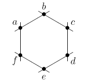
There is no line containing a pair of points here except when a line is actually shown, and more generally there are no 'shortcuts' beyond what is shown. For example, we go from \( a\) to \( b\) by following just one line, but it takes two to get from \( a\) to \( c,\) and three to get from \( a\) to \( d.\)
Betty Salzberg wrote a nice introduction to these ideas in 1982. Among other things, she noted that the points and lines in the incidence geometry of the split real form of G2 correspond to 1- and 2-dimensional null subalgebras of the imaginary split octonions. This was shown by Tits in 1955.
In 1993, Bryant and Hsu gave a detailed treatment of curves in manifolds equipped with 2-dimensional distributions, greatly extending the work of Cartan:
• Robert Bryant and Lucas Hsu, Rigidity of integral curves of rank 2 distributions.
They showed how the space of configurations of one surface rolling on another fits into this framework. However, Igor Zelenko may have been the first to explicitly mention a ball rolling on another ball in this context, and to note that something special happens when their ratio of radii is 3 or 1/3. In a 2004 paper, he considered an invariant of (2,3,5) distributions. He calculated it for the distribution arising from a ball rolling on a larger ball and showed it equals zero in these two cases.
• Igor Zelenko, Variational approach to differential invariants of rank 2 vector distributions.
(In our paper, John Huerta and I assume that the rolling ball is smaller than the fixed one, simply to eliminate one of these cases and focus on the case where the fixed ball is 3 times as big.)
In 2006, Bor and Montgomery's paper put many of the pieces together. They studied the (2,3,5) distribution on \( S^2 \times \mathrm{SO}(3)\) coming from a ball of radius 1 rolling on a ball of radius R, and proved a theorem which they credit to Robert Bryant. First, passing to the double cover, they showed the corresponding distribution on \( S^2 \times \mathrm{SU}(2)\) has a symmetry group whose identity component contains the split real form of G2 when R = 3 or 1/3. Second, they showed this action does not descend to original rolling ball configuration space \( S^2 \times \mathrm{SO}(3).\) Third, they showed that for any other value of R except R = 1, the symmetry group is isomorphic to \( \mathrm{SU}(2) \times \mathrm{SU}(2)/\pm(1,1).\) They also wrote:
Despite all our efforts, the "3" of the ratio 1:3 remains mysterious. In this article it simply arises out of the structure constants for G2 and appears in the construction of the embedding of \( \mathfrak{so}(3) \times \mathfrak{so}(3)\) into \( \mathfrak{g}_2.\) Algebraically speaking, this "3" traces back to the 3 edges in \( \mathfrak{g}_2\)'s Dynkin diagram and the consequent relative positions of the long and short roots in the root diagram for \( \mathfrak{g}_2\) which the Dynkin diagram is encoding.Open problem. Find a geometric or dynamical interpretation for the "3" of the 3:1 ratio.
As you can see from what I've said, John Huerta and I have offered a solution to this puzzle: the "3" comes from the fact that a ball rolling once around a ball 3 times as big turns around exactly 4 times—just what you need to get a relationship to a spinorial ball rolling on a projective plane, and thus the lightcone in the split octonions! The most precise statement of this explanation comes in Theorem 3 of our paper.
While Bor and Montgomery's paper goes into considerable detail about the connection with split octonions, most of their work uses the now standard technology of semisimple Lie algebras: roots, weights and the like. In 2006, Sagerschnig described the incidence geometry of \( \mathrm{G}_2\) using the split octonions, and in 2008, Agrachev wrote a paper entitled 'Rolling balls and octonions'. He emphasizes that the double cover \( S^2 \times \mathrm{SU}(2)\) can be identified with the double cover of \( \mathrm{PC}\), the projectivization of the set of null vectors in the imaginary split octonions. He then shows that given a point \( \langle x \rangle \in \mathrm{PC},\) the set of points \( \langle y \rangle\) connected to \( \langle x \rangle\) by a single roll is the annihilator
$$ \{ x \in \mathbb{I} : y x = 0 \} $$
where \( \mathbb{I}\) is the space of imaginary split octonions.
This sketch of the history is incomplete in many ways. As usual, history resembles a fractal: the more closely you study it, the more details you see! If you want to dig deeper, I strongly recommend these:
• Ilka Agricola, Old and new on the the exceptional group G2.
• Robert Bryant, Élie Cartan and geometric duality.
This paper is also very helpful and fun:
• Aroldo Kaplan, Quaternions and octonions in mechanics.
It emphasizes the role that quaternions play in describing rotations, and the way an imaginary split octonion is built from an imaginary quaternion and a quaternion. And don't forget this:
• Andrei Agrachev, Rolling balls and octonions.
Have fun! And make sure to watch the animation of a rolling ball in the next and final part of this series.
You can also read comments on Azimuth, and make your own comments or ask questions there!
|
|
|
|