


|
|
|
|
Here's a puzzle. Guess the next term of this sequence:
and then guess the meaning of this sequence! I'll give away the answer after telling you about Coleman's videos on quantum field theory and an amazing result on the homotopy groups of spheres.
But first... the astronomy picture of the day.
The Eaton Collection at UC Riverside may be the world's best library of science fiction:
1) The Eaton Collection of Science Fiction, Fantasy, Horror and Utopian Literature, http://eaton-collection.ucr.edu/.
Right now my wife Lisa Raphals is attending a conference there on the role of Mars in SF, called "Chronicling Mars". Gregory Benford, Frederik Pohl, Greg Bear, David Brin, Kim Stanley Robinson and even Ray Bradbury are all there! But for some reason I'm staying home working on This Week's Finds. I'd say that shows true devotion - or maybe just stupidity.
Anyway, in honor of the occasion, here's an incredible closeup of a crater on Mars' moon Phobos:
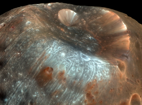
2) Astronomy Picture of the Day, Stickney Crater http://apod.nasa.gov/apod/ap080410.html
It's another great example of how machines in space now deliver many more thrills per buck than the old-fashioned approach using canned primates. This photo was taken by HiRISE, the High Resolution Imaging Science Experiment - the same satellite that took the stunning photos of Martian dunes which graced "week262".
Mars has two moons, Phobos and the even tinier Deimos. Their names mean "fear" and "dread" in Greek, since in Greek mythology they were sons of Mars (really Ares), the god of war.
Interestingly, Kepler predicted that Mars had two moons before they were seen. This sounds impressive, but it was simple interpolation, since Earth has 1 moon and Jupiter has 4. Or at least Galileo saw 4 - now we know there are a lot more.
Phobos is only 21 kilometers across, and the big crater you see here - Stickney Crater - is about 9 kilometers across. That's almost half the size of the whole moon! The collision that created it must have almost shattered Phobos.
Phobos is so light - just twice the density of water - that people once thought it might be hollow. This now seems unlikely, though it's been the premise of a few SF stories. It's more likely that Phobos is a loosely packed pile of carbonaceous chondrites captured from the asteroid belt.
Phobos orbits so close to Mars that it zips around once every 8 hours, faster than Mars itself rotates! Oddly, in 1726 Jonathan Swift wrote about two moons of Mars in his novel "Gulliver's Travels" - and he guessed that the inner one orbited Mars every 10 hours.
Gravitational tidal forces are dragging Phobos down, so in only 10 million years it'll either crash or - more likely - be shattered by tidal forces and form a ring of debris.
So, enjoy it while it lasts.
Anyone who's seriously struggled to master quantum field theory is likely to have profited from this book:
3) Sidney Coleman, Aspects of Symmetry: Selected Erice Lectures, Cambridge U. Press, Cambridge, 1988.
It's brimming with wisdom and humor. You should have already encountered quantum field theory before trying it: what you'll get are deeper insights.
But what if you're just getting started?
Sidney Coleman, recently deceased, was one of the best quantum field theorists from the heyday of particle physics. As a grad student I took a course on quantum field theory from Eddie Farhi, who said he based his class on the notes from Coleman's class at Harvard. So, I've always been curious about these notes. Now they're available online in handwritten form:
4) Sidney Coleman, lecture notes on quantum field theory, transcribed by Brian Hill, http://www.damtp.cam.ac.uk/user/dt281/qft/col1.pdf and http://www.damtp.cam.ac.uk/user/dt281/qft/col2.pdf
Someone should LaTeX them up!
Even more fun, you can now see videos of Coleman teaching quantum field theory:
5) Sidney Coleman, Physics 253: Quantum Field Theory, 50 lectures recorded 1975-1976, http://www.physics.harvard.edu/about/Phys253.html
This is a younger, hipper Coleman than I'd ever seen: long-haired, sometimes puffing on a cigarette between sentences. He begins by saying "Umm... this is Physics 253, a course in relativistic quantum mechanics. My name is Sidney Coleman. The apparatus you see around you is part of a CIA surveillance project."
I wish I'd had access to these when I was a kid!
Now for some miraculous math. Daniel Moskovich kindly pointed out a paper that describes all the homotopy groups of the 2-sphere, and I want to summarize the main result.
I explained the idea of homotopy groups back in "week102". Very roughly, the nth homotopy group of a space X, usually denoted πn(X), is the set of ways you can map an n-sphere into that space, where we count two ways as the same if you can continuously deform one to the other. If a space has holes, homotopy groups are one way to detect those holes.
Homotopy groups are notoriously hard to compute - so even for so humble a space as the 2-sphere, S2, there's a sense in which "nobody knows" all its homotopy groups. People know the first 64, though. Here are a few:
π1(S2) = 0
π2(S2) = Z
π3(S2) = Z
π4(S2) = Z/2
π5(S2) = Z/2
π6(S2) = Z/4 × Z/3
π7(S2) = Z/2
π8(S2) = Z/2
π9(S2) = Z/3
π10(S2) = Z/3 × Z/5
π11(S2) = Z/2
π12(S2) = Z/2 × Z/2
π13(S2) = Z/2 × Z/2 × Z/3
π14(S2) = Z/2 × Z/2 × Z/4 × Z/3 × Z/7
π15(S2) = Z/2 × Z/2
Apart from the fact that they're all abelian groups, all finite except for the first two, it's hard to spot any pattern!
In fact there's a majestic symphony of patterns in the homotopy groups of spheres, starting from ones that are easy to explain and working on up to those that push the frontiers of mathematics, like elliptic cohomology. But, many of these patterns are too complex for present-day mathematics until we use some tricks to "water down" or simplify the homotopy groups.
So, what people often do first is take the limit of πn+k(Sn) as n → ∞, getting what's called the kth "stable" homotopy group of spheres. It's a wonderful but well-understood fact that these limits really exist. But so far, even these are too complicated to understand until we work "at a prime p". This means that we take the kth stable homotopy group of spheres and see which groups of the form Z/pn show up in it. For example,
π14(S2) = Z/2 × Z/2 × Z/4 × Z/3 × Z/7
but if we work "at the prime 2" we just see the Z/2 × Z/2 × Z/4.
After all this data processing, we get some astounding pictures:
This picture summarizes the first 999 stable homotopy groups of spheres at the prime 5. To understand exactly what it means, read this:
6) Allen Hatcher, Stable homotopy groups of spheres, http://www.math.cornell.edu/~hatcher/stemfigs/stems.html
Order teetering on the brink of chaos! If you're brave, you can learn more about this stuff here:
7) Douglas C. Ravenel, Complex Cobordism and Stable Homotopy Groups of Spheres, AMS, Providence, Rhode Island, 2003.
If you're less brave, I strongly suggest starting here:
8) Wikipedia, Homotopy groups of spheres, http://en.wikipedia.org/wiki/Homotopy_groups_of_spheres
But now, I want to talk about an amazing paper that pursues a very different line of attack. It gives a beautiful description of all the homotopy groups of S2, in terms of braids:
9) A. Berrick, F. R. Cohen, Y. L. Wong and J. Wu, Configurations, braids and homotopy groups, J. Amer. Math. Soc., 19 (2006), 265-326. Also available at http://www.math.nus.edu.sg/~matwujie/BCWWfinal.pdf
For this you need to realize that for any n, there's a group Bn whose elements are n-strand braids. For example, here's an element of B3:
|   |  |
 \ /   |
  /    |
 / \   |
|   \ /
|    /
|   / \
 \ /   |
  /    |
 / \   |
|   \ /
|    /
|   / \
 \ /   |
  /    |
 / \   |
|   \ /
|    /
|   / \
|  |   |
I actually talked about this specific braid back in "week233". But anyway, we count two braids as the same if you can wiggle one around until it looks like the other without moving the ends at the top and bottom - which you can think of as nailed to the ceiling and floor.
How do braids become a group? Easy: we multiply them by putting one on top of the other. For example, this braid:
     |   |   |
      \ /    |
A  =   /     |
      / \    |
     |   |   |
times this one:
     |   |   |
     |    \ /
B =  |     /
     |    / \
     |   |   |
equals this:
     |   |   |
      \ /    |
       /     |
      / \    |
     |   |   |
AB = |   |   |
     |    \ /
     |     /
     |    / \
     |   |   |
and in fact the big one I showed you earlier is (AB)3.
As you let your eye slide from the top to the bottom of a braid, the strands move around. We can visualize their motion as a bunch of points running around the plane, never bumping into each other. This gives an interesting way to generalize the concept of a braid! Instead of points running around the plane, we can have points running around S2, or some other surface X. So, for any surface X and any number n of strands, we get a "surface braid group", called Bn(X).
As I hinted in "week261", these surface braid groups have cool relationships to Dynkin diagrams. I urged you to read this paper, and I'll urge you again:
10) Daniel Allcock, Braid pictures for Artin groups, available as arXiv:math.GT/9907194.
But for now, we just need the "spherical braid group" Bn(S2) together with the usual braid group Bn.
Let's say a braid is "Brunnian" if when you remove any one strand, the remaining braid becomes the identity: you can straighten out all the remaining strands to make them vertical. It's a fun little exercise to check that Brunnian braids form a subgroup of all braids. So, we have an n-strand Brunnian braid group BBn.
The same idea works for braids on other surface, like the 2-sphere. So, we also have an n-strand spherical Brunnian braid group BBn(S2).
Now, there's obvious map
Bn → Bn(S2)
Why? An element of Bn describes the motion of a bunch of points running around the plane, but the plane sits inside the 2-sphere: the 2-sphere is just the plane with an extra point tacked on. So, an ordinary braid gives a spherical braid.
This map clearly sends Brunnian braids to spherical Brunnian braids, so we get a map
f: BBn → BBn(S2)
And now we're ready for the shocking theorem of Berrick, Cohen, Wong and Wu:
Theorem: For n > 3, πn(S2) is BBn(S2) modulo the image of f.
In something more like plain English: when n is big enough, the nth homotopy group of the 2-sphere consists of spherical Brunnian braids modulo ordinary Brunnian braids!
Zounds! What do the homotopy groups of S2 have to do with braids? It's not supposed to be obvious! The proof of this result is long and deep, making use of flows on metric spaces, and also the fact that all the Brunnian braid groups BBn fit together into a "simplicial group" whose nth homology is the nth homotopy group of S2. I'd love to understand all this stuff, but I don't yet.
This result doesn't instantly help us "compute" the homotopy groups of S2 - at least not in the sense of writing them down as a product of groups like Z/pn. But, it gives a new view of these homotopy groups, and there's no telling where this might lead.
When I was first getting ready to write this article, I was also going to tell you about some amazing descriptions of the homotopy groups of the 3-sphere, due to Wu.
However, I later realized - first to my shock, and then my embarrassment for not having known it already - that the nth homotopy group of S3 is the same as the nth homotopy group of S2, at least for n > 2. Do you see why?
Given this, it turns out that Wu's results are predecessors of the theorem just stated, a bit more combinatorial and less "geometric". Wu's results appeared here:
12) Jie Wu, On combinatorial descriptions of the homotopy groups of certain spaces, Math. Proc. Camb. Phil. Soc. 130 (2001), 489-513. Also available at http://www.math.nus.edu.sg/~matwujie/newnewpis_3.pdf
Jie Wu, A braided simplicial group, Proc. London Math. Soc. 84 (2002), 645-662. Also available at http://www.math.nus.edu.sg/~matwujie/wgroup05-19-01.pdf
and there's a nice summary of these results on his webpage:
13) Jie Wu, 2.1 Homotopy groups and braids, halfway down the page at http://www.math.nus.edu.sg/~matwujie/Research2.html
See also this expository paper:
14) Fred R. Cohen and Jie Wu, On braid groups and homotopy groups, Geometry & Topology Monographs 13 (2008), 169-193. Also available at http://www.math.nus.edu.sg/~matwujie/cohen.wu.GT.revised.29.august.2007.pdf
Next I want to talk about puzzle mentioned at the start of this Week's Finds... but first I should answer the puzzle I just raised. Why do the homotopy groups of S2 match those of S3 after a while? Because of the Hopf fibration! This is a fiber bundle with S3 as total space, S2 as base space and S1 as fiber:
S1 → S3 → S2
Like any fiber bundle, it gives a long exact sequence of homotopy groups as explained in "week151":
... → πn(S1) → πn(S3) → πn(S2) → πn-1(S1) → ...
but the homotopy groups of S1 vanishes after the first, so we get
... → 0 → πn(S3) → πn(S2) → 0 → ...
for n > 2, which says that
πn(S3) ≅ πn(S2)
Okay, now for this mysterious sequence:
The next term is obviously 7. If you guessed anything else, you were over-analyzing. So the real question is: why the funny "hiccup" at the beginning? Why the repeated 1?
You'll find two explanations of this sequence in Sloane's Online Encyclopedia of Integer Sequences, but neither of them is the reason James Dolan and I ran into it. We were learning about theta functions...
Say you have a torus. Then the complex line bundles over it are classified by an integer called their "first Chern number". In some sense, this integer this measures how "twisted" the bundle is. For example, you can put any connection on the bundle, compute its curvature 2-form, and integrate it over the torus: up to some constant factor, you'll get the first Chern number.
A torus is a 2-dimensional manifold, but we can also make it into a 1-dimensional complex manifold, often called an "elliptic curve". In fact we can do this in infinitely many fundamentally different ways, one for each point in the "moduli space of elliptic curves". I've explained this repeatedly here - try "week125" for a good starting-point - so I won't do so again. The details don't really matter here.
Back to line bundles. If we pick an elliptic curve, we can try to classify the holomorphic complex line bundles over it - that is, those where the transition functions are holomorphic (or in other words, complex-analytic). Here the classification is subtler. It turns out you need, not just the first Chern number, which is discrete, but another parameter which can vary in a continuous way.
Interestingly, this other parameter can be thought of as just a point on your elliptic curve! So, an elliptic curve is a space that classifies holomorphic line bundles over itself - at least, those with fixed first Chern number. Curiously circular, eh? This is just one of several curiously circular classification theorems that happen in this game...
But I'm actually digressing a bit - I'm having trouble resisting the temptation to explain everything I've just been learning, since it's so simple and beautiful. Don't worry - all you need to know is that holomorphic line bundles over an elliptic curve are classified by an integer and some other continuous parameter.
The puzzle then arises: how many holomorphic sections do these line bundles have? More precisely: what's the dimension of the space of holomorphic sections?
Before I answer this, I can't resist adding that these holomorphic sections have a long and illustrious history - they're called "theta functions", and you can learn about them here:
15) Jun-ichi Igusa, Theta Functions, Springer, Berlin, 1972.
16) David Mumford, Tata Lectures on Theta, 3 volumes, Birkhauser, Boston, 1983-1991.
They're important in geometric quantization, where holomorphic sections of line bundles describe states of quantum systems, and the reciprocal of the first Chern number is proportional to Planck's constant. In fact, I first ran into theta functions years ago, when trying to quantize a black hole - see the end of "week112" for more details.
But anyway, here's the answer to the puzzle. The dimension turns out not to depend on the continuous parameter labelling our line bundle, but only on its first Chern number. If that number is negative, the dimension is 0. But if it's 0,1,2,3,4,5,6 and so on, the dimension goes like this:
Now, this sequence is fairly weird, because of the extra "1" at the beginning. I hadn't noticed this back when I was quantizing black holes, because the extra "1" happens for first Chern number zero, which would correspond to Planck's constant being infinite. But now that I'm just thinking about math, it sticks out like a sore thumb!
It's got to be right, since the line bundle with first Chern number zero is the trivial bundle, its sections are just functions, and the only holomorphic functions on a compact complex manifold are constants - so there's a 1-dimensional space of them. But, it's weird.
Luckily, Jim figured out the explanation for this sequence. First of all, we can encode it into a power series:
1 + x + 2x2 + 3x3 + 4x4 + ...which we can rewrite as a rational function:
                                       (1-x6)
1 + x + 2x2 + 3x3 + 4x4 + ...  =  ------------------
                                  (1-x)(1-x2)(1-x3)
Now, the reason for doing this is that we can pick a line bundle of first Chern number 1, say L, and get a line bundle of any Chern number n by taking the nth tensor power of L - let's call that L⊗n. We can multiply a section of L⊗n and a section of L⊗m to get a section of L⊗(n+m). So, all these spaces of sections we're studying fit together to form a commutative graded ring! And, whenever you have a graded ring, it's a good idea to write down a power series that encodes the dimensions of each grade, just as we've done above. This is called a "Poincare series".
And, when you have a commutative graded ring with one generator of degree 1, one generator of degree 2, one generator of degree 3, one relation of degree 6, and no "relations between relations" (or "syzygies"), its Poincare series will be
        (1-x6)
  ------------------
  (1-x1)(1-x2)(1-x3)
That's how it always works - think about it.
So, it's natural to hope that our ring built from holomorphic sections of all the line bundles L⊗n will have one generator of degree 1, one of degree 2, one of degree 3, and one relation of degree 6.
And, this seems to be true!
As I mentioned, people usually call these holomorphic sections "theta functions". So, what we're getting is a description of the ring of theta functions in terms of generators and relations.
How does it work, exactly? Well, I must admit I'm not quite sure. Jim has some ideas, but it seems I need to do something a bit different to get his story to work for me. Maybe it goes something like this. We can write any elliptic curve as the solutions of this equation:
y2 = x3 + Bx + C
for certain constants B and C that depend on the elliptic curve. (See "week13" and "week261" for details.) Now, this equation is not homogeneous in the variables y and x, but we can think of it as homogeneous in a sneaky sense if we throw in an extra variable like this:
y2 = x3 + Bxz4 + Cz6
and decree that:
y has grade 3
x has grade 2
z has grade 1
Then all the terms in the equation have grade 6. So, we're getting a commutative graded ring with generators of degree 1, 2, and 3 and a relation of grade 6. And, I'm hoping this ring consists of algebraic functions on the total space of some line bundle L* over our elliptic curve. z should be a function that's linear in the fiber directions, hence a section of L. x should be quadratic in the fiber directions, hence a section of L⊗2. And y should be cubic, hence a section of L⊗3. If L has first Chern number 1, I think we're in business.
If anybody knows about this stuff, I'd appreciate corrections or references.
There's a lot more to say about this business... because it's all part of a big story about elliptic curves, theta functions and modular forms. But, I want to quit here for now.
Addenda: I thank David Corfield for pointing out how to get ahold of Wu's papers free online - and earlier, for telling me Wu's combinatorial description of π3(S2).
Martin Ouwehand told me that some of Coleman's lecture notes on quantum field theory are available in TeX here:
17) Sidney Coleman, Quantum Field Theory, first 11 lectures notes TeXed by Bryan Gin-ge Chen, available at http://www.physics.upenn.edu/~chb/phys253a/coleman/
James Dolan pointed out that this article:
18) Wikipedia, Riemann-Roch theorem, http://en.wikipedia.org/wiki/Riemann-Roch
has some very relevant information on the sequence
though it's phrased not in terms of "sections of line bundles", but instead in terms of "divisors" (secretly another way of talking about the same thing). Let me quote a portion, just to whet your interest:
We start with a connected compact Riemann surface of genus g, and a fixed point P on it. We may look at functions having a pole only at P. There is an increasing sequence of vector spaces: functions with no poles (i.e., constant functions), functions allowed at most a simple pole at P, functions allowed at most a double pole at P, a triple pole, ... These spaces are all finite dimensional. In case g = 0 we can see that the sequence of dimensions starts
1, 2, 3, ...This can be read off from the theory of partial fractions. Conversely if this sequence starts
1, 2, ...then g must be zero (the so-called Riemann sphere).In the theory of elliptic functions it is shown that for g = 1 this sequence is
1, 1, 2, 3, 4, 5 ...and this characterises the case g = 1. For g > 2 there is no set initial segment; but we can say what the tail of the sequence must be. We can also see why g = 2 is somewhat special.
The reason that the results take the form they do goes back to the formulation (Roch's part) of the [Riemann-Roch] theorem: as a difference of two such dimensions. When one of those can be set to zero, we get an exact formula, which is linear in the genus and the degree (i.e. number of degrees of freedom). Already the examples given allow a reconstruction in the shape
dimension - correction = degree - g + 1.For g = 1 the correction is 1 for degree 0; and otherwise 0. The full theorem explains the correction as the dimension associated to a further, 'complementary' space of functions.
You can see more discussion of this Week's Finds at the n-Category Café.
The career of a young theoretical physicist consists of treating the harmonic oscillator in ever-increasing levels of abstraction. - Sidney Coleman
© 2008 John Baez
baez@math.removethis.ucr.andthis.edu
|
|
|
|