

|
|
|
|
In chemistry a type of atom, molecule, or ion is called a chemical species, or species for short. Since we're applying our ideas to both chemistry and biology, it's nice that 'species' is also used for a type of organism in biology. This stochastic Petri net describes the simplest reversible reaction of all, involving two species:
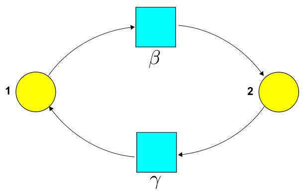
We have species 1 turning into species 2 with rate constant $ \beta,$ and species 2 turning back into species 1 with rate constant $ \gamma.$ So, the rate equation is:
$$ \begin{array}{ccc} \displaystyle{ \frac{d x_1}{d t} } &=& -\beta x_1 + \gamma x_2 \\ \qquad \mathbf{} \\ \displaystyle{ \frac{d x_2}{d t} } &=& \beta x_1 - \gamma x_2 \end{array} $$where $ x_1$ and $ x_2$ are the amounts of species 1 and 2, respectively.
Let's look for equilibrium solutions of the rate equation, meaning solutions where the amount of each species doesn't change with time. Equilibrium occurs when each species is getting created at the same rate at which it's getting destroyed.
So, let's see when
$$ \displaystyle{ \frac{d x_1}{d t} = \frac{d x_2}{d t} = 0 } $$Clearly this happens precisely when
$$ \beta x_1 = \gamma x_2 $$This says the rate at which 1's are turning into 2's equals the rate at which 2's are turning back into 1's. That makes perfect sense.
In general, a chemical reaction involves a bunch of species turning into a bunch of species. Since 'bunch' is not a very dignified term, a bunch of species is usually called a complex. We saw last time that it's very interesting to study a strong version of equilibrium: complex balanced equilibrium, in which each complex is being created at the same rate at which it's getting destroyed. However, in the Petri net we're studying today, all the complexes being produced or destroyed consist of a single species. In this situation, any equilibrium solution is automatically complex balanced. This is great, because it means we can apply the Anderson-Craciun-Kurtz theorem from last time! This says how to get from a complex balanced equilibrium solution of the rate equation to an equilibrium solution of the master equation.
First remember what the master equation says. Let $ \psi_{n_1, n_2}(t)$ be the probability that we have $ n_1$ things of species 1 and $ n_2$ things of species 2 at time $ t$. We summarize all this information in a formal power series:
$$ \Psi(t) = \sum_{n_1, n_2 = 0}^\infty \psi_{n_1, n_2}(t) z_1^{n_1} z_2^{n_2} $$Then the master equation says
$$ \frac{d}{d t} \Psi(t) = H \Psi (t) $$where following the general rules laid down in Part 8,
$$ \begin{array}{ccl} H &=& \beta (a_2^\dagger - a_1^\dagger) a_1 + \gamma (a_1^\dagger - a_2^\dagger )a_2 \end{array} $$This may look scary, but the annihilation operator $ a_i$ and the creation operator $ a_i^\dagger$ are just funny ways of writing the partial derivative $ \partial/\partial z_i$ and multiplication by $ z_i$, so
$$ \begin{array}{ccl} H &=& \displaystyle{ \beta (z_2 - z_1) \frac{\partial}{\partial z_1} + \gamma (z_1 - z_2) \frac{\partial}{\partial z_2} } \end{array} $$or if you prefer,
$$ \begin{array}{ccl} H &=& \displaystyle{ (z_2 - z_1) \, (\beta \frac{\partial}{\partial z_1} - \gamma \frac{\partial}{\partial z_2}) } \end{array} $$The first term describes species 1 turning into species 2. The second describes species 2 turning back into species 1.
Now, the Anderson-Cranciun-Kurtz theorem says that whenever $ (x_1,x_2)$ is a complex balanced solution of the rate equation, this recipe gives an equilibrium solution of the master equation:
$$ \displaystyle{ \Psi = \frac{e^{x_1 z_1 + x_2 z_2}}{e^{x_1 + x_2}} } $$In other words: whenever $ \beta x_1 = \gamma x_2$, we have
we have
$$ H\Psi = 0 $$ Let's check this! For starters, the constant in the denominator of $ \Psi$ doesn't matter here, since $ H$ is linear. It's just a normalizing constant, put in to make sure that our probabilities $ \psi_{n_1, n_2}$ sum to 1. So, we just need to check that $$ \displaystyle{ (z_2 - z_1) (\beta \frac{\partial}{\partial z_1} - \gamma \frac{\partial}{\partial z_2}) e^{x_1 z_1 + x_2 z_2} = 0 } $$If we do the derivatives on the left hand side, it's clear we want
$$ \displaystyle{ (z_2 - z_1) (\beta x_1 - \gamma x_2) e^{x_1 z_1 + x_2 z_2} = 0 } $$And this is indeed true when $ \beta x_1 = \gamma x_2 $.
So, the theorem works as advertised. And now we can work out the probability $ \psi_{n_1,n_2}$ of having $ n_1$ things of species 1 and $ n_2$ of species 2 in our equilibrium state $ \Psi$. To do this, we just expand the function $ \Psi$ as a power series and look at the coefficient of $ z_1^{n_1} z_2^{n_2}$. We have
$$ \Psi = \displaystyle{ \frac{e^{x_1 z_1 + x_2 z_2}}{e^{x_1 + x_2}} } = \displaystyle{ \frac{1}{e^{x_1} e^{x_2}} \sum_{n_1,n_2}^\infty \frac{(x_1 z_1)^{n_1}}{n_1!} \frac{(x_2 z_2)^{n_2}}{n_2!} } $$so we get
$$ \psi_{n_1,n_2} = \displaystyle{ \frac{1}{e^{x_1}} \frac{x_1^{n_1}}{n_1!} \; \cdot \; \frac{1}{e^{x_2}} \frac{x_1^{n_2}}{n_2!} }$$This is just a product of two independent Poisson distributions!
In case you forget, a Poisson distribution says the probability of $ k$ events occurring in some interval of time if they occur with a fixed average rate and independently of the time since the last event. If the expected number of events is $ \lambda$, the Poisson distribution is
$$ \displaystyle{ \frac{1}{e^\lambda} \frac{\lambda^k}{k!} } $$and it looks like this for various values of $ \lambda$:
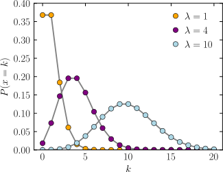
It looks almost like a Gaussian when $ \lambda$ is large, but when $ \lambda$ is small it becomes very lopsided.
Anyway: we've seen that in our equilibrium state, the number of things of species $ i = 1,2$ is given by a Poisson distribution with mean $ x_i$. That's very nice and simple... but the amazing thing is that these distributions are independent.
Mathematically, this means we just multiply them to get the probability of finding $ n_1$ things of species 1 and $ n_2$ of species 2. But it also means that knowing how many things there are of one species says nothing about the number of the other.
But something seems odd here. One transition in our Petri net consumes a 1 and produces a 2, while the other consumes a 2 and produces a 1. The total number of particles in the system never changes. The more 1's there are, the fewer 2's there should be. But we just said knowing how many 1's we have tells us nothing about how many 2's we have!
At first this seems like a paradox. Have we made a mistake? Not exactly. But we're neglecting something.
Namely: the equilibrium solutions of the master equation we've found so far are not the only ones! There are other solutions that fit our intuitions better.
Suppose we take any of our equilibrium solutions $ \Psi$ and change it like this: set the probability $ \psi_{n_1,n_2}$ equal to 0 unless
$$ n_1 + n_2 = n $$but otherwise leave it unchanged. Of course the probabilities no longer sum to 1, but we can rescale them so they do.
The result is a new equilibrium solution, say $ \Psi_n.$ Why? Because, as we've already seen, no transitions will carry us from one value of $ n_1 + n_2$ to another. And in this new solution, the number of 1's is clearly not independent from the number of 2's. The bigger one is, the smaller the other is.
Puzzle 1. Show that this new solution $ \Psi_n$ depends only on $ n$ and the ratio $ x_1/x_2 = \gamma/\beta$, not on anything more about the values of $ x_1$ and $ x_2$ in the original solution
$$ \Psi = \displaystyle{ \frac{e^{x_1 z_1 + x_2 z_2}}{e^{x_1 + x_2}} } $$Puzzle 2. What is this new solution like when $ \beta = \gamma$? (This particular choice makes the problem symmetrical when we interchange species 1 and 2.)
What's happening here is that this particular stochastic Petri net has a 'conserved quantity': the total number of things never changes with time. So, we can take any equilibrium solution of the master equation and—in the language of quantum mechanics—`project down to the subspace' where this conserved quantity takes a definite value, and get a new equilibrium solution. In the language of probability theory, we say it a bit differently: we're 'conditioning on' the conserved quantity taking a definite value. But the idea is the same.
This important feature of conserved quantities suggests that we should try to invent a new version of Noether's theorem. This theorem links conserved quantities and symmetries of the Hamiltonian.
There are already a couple versions of Noether's theorem for classical mechanics, and for quantum mechanics... but now we want a version for stochastic mechanics. And indeed one exists, and it's relevant to what we're doing here. We'll show it to you next time.
You can also read comments on Azimuth, and make your own comments or ask questions there!
|
|
|
|