October 4, 2011

Network Theory (Part 11)

John Baez and Brendan Fong

Noether proved lots of theorems, but when people talk about Noether's theorem, they always seem to mean her result linking symmetries to conserved quantities. Her original result applied to classical mechanics, but today we'd like to present a version that applies to 'stochastic mechanics'—or in other words, Markov processes.

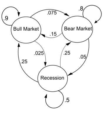
What's a Markov process? We'll say more in a minute—but in plain English, it's a physical system where something hops around randomly from state to state, where its probability of hopping anywhere depends only on where it is now, not its past history. Markov processes include, as a special case, the stochastic Petri nets we've been talking about.

Our stochastic version of Noether's theorem is copied after a well-known quantum version. It's yet another example of how we can exploit the analogy between stochastic mechanics and quantum mechanics. But for now we'll just present the stochastic version. Next time we'll compare it to the quantum one.

Markov processes

We should and probably will be more general, but let's start by considering a finite set of states, say $X$. To describe a Markov process we then need a matrix of real numbers $H = (H_{i j})_{i, j \in X}.$ The idea is this: suppose right now our system is in the state $i$. Then the probability of being in some state $j$ changes as time goes by—and $H_{i j}$ is defined to be the time derivative of this probability right now.

So, if $\psi_i(t)$ is the probability of being in the state $i$ at time $t$, we want the master equation to hold:

$$ \frac{d}{d t} \psi_i(t) = \sum_{j \in X} H_{i j} \psi_j(t) $$

This motivates the definition of 'infinitesimal stochastic', which we recall from Part 5:

Definition. Given a finite set $X$, a matrix of real numbers $H = (H_{i j})_{i, j \in X}$ is infinitesimal stochastic if

and

$$ \sum_{i \in X} H_{i j} = 0 $$

for all $j \in X$.

The inequality says that if we start in the state $i$, the probability of being in some other state, which starts at 0, can't go down, at least initially. The equation says that the probability of being somewhere or other doesn't change. Together, these facts imply that:

$$ H_{i i} \le 0 $$

That makes sense: the probability of being in the state $i$, which starts at 1, can't go up, at least initially.

Using the magic of matrix multiplication, we can rewrite the master equation as follows:

$$ \frac{d}{d t} \psi(t) = H \psi(t) $$

and we can solve it like this:

$$ \psi(t) = \exp(t H) \psi(0) $$

If $H$ is an infinitesimal stochastic operator, we will call $\exp(t H)$ a Markov process, and $H$ its Hamiltonian.

(Actually, most people call $\exp(t H)$ a Markov semigroup, and reserve the term Markov process for another way of looking at the same idea. So, be careful.)

Noether's theorem is about 'conserved quantities', that is, observables whose expected values don't change with time. To understand this theorem, you need to know a bit about observables. In stochastic mechanics an observable is simply a function assigning a number $O_i$ to each state $i \in X$.

However, in quantum mechanics we often think of observables as matrices, so it's nice to do that here, too. It's easy: we just create a matrix whose diagonal entries are the values of the function $O$. And just to confuse you, we'll also call this matrix $O$. So:

$$ O_{i j} = \left\{ \begin{array}{ccl} O_i & \textrm{if} & i = j \\ 0 & \textrm{if} & i \neq j \end{array} \right. $$

One advantage of this trick is that it lets us ask whether an observable commutes with the Hamiltonian. Remember, the commutator of matrices is defined by

$$ [O,H] = O H - H O$$

Noether's theorem will say that $[O,H] = 0$ if and only if $O$ is 'conserved' in some sense. What sense? First, recall that a stochastic state is just our fancy name for a probability distribution $\psi$ on the set $X$. Second, the expected value of an observable $O$ in the stochastic state $\psi$ is defined to be

$$ \sum_{i \in X} O_i \psi_i $$

In Part 5 we introduced the notation

$$ \int \phi = \sum_{i \in X} \phi_i $$

for any function $\phi$ on $X$. The reason is that later, when we generalize $X$ from a finite set to a measure space, the sum at right will become an integral over $X$. Indeed, a sum is just a special sort of integral!

Using this notation and the magic of matrix multiplication, we can write the expected value of $O$ in the stochastic state $\psi$ as

$$ \int O \psi $$

We can calculate how this changes in time if $\psi$ obeys the master equation... and we can write the answer using the commutator $[O,H]$:

Lemma. Suppose $H$ is an infinitesimal stochastic operator and $O$ is an observable. If $\psi(t)$ obeys the master equation, then

$$ \frac{d}{d t} \int O \psi(t) = \int [O,H] \psi(t) $$

Proof. Using the master equation we have

\[ \frac{d}{d t} \int O \psi(t) = \int O \frac{d}{d t} \psi(t) = \int O H \psi(t) \]

But since $H$ is infinitesimal stochastic,

$$ \sum_{i \in X} H_{i j} = 0 $$

so for any function $\phi$ on $X$ we have

$$ \int H \phi = \sum_{i, j \in X} H_{i j} \phi_j = 0 $$

and in particular

\[ \int H O \psi(t) = 0 \]

Since $[O,H] = O H - H O $, we conclude from (1) and (2) that

$$ \frac{d}{d t} \int O \psi(t) = \int [O,H] \psi(t) $$

as desired.   █

The commutator doesn't look like it's doing much here, since we also have

$$ \frac{d}{d t} \int O \psi(t) = \int O H \psi(t) $$

which is even simpler. But the commutator will become useful when we get to Noether's theorem!

Noether's theorem

Here's a version of Noether's theorem for Markov processes. It says an observable commutes with the Hamiltonian iff the expected values of that observable and its square don't change as time passes:

Theorem. Suppose $H$ is an infinitesimal stochastic operator and $O$ is an observable. Then $$ [O,H] =0 $$

if and only if

$$ \frac{d}{d t} \int O\psi(t) = 0 $$

and

$$ \frac{d}{d t} \int O^2\psi(t) = 0 $$

for all $\psi(t)$ obeying the master equation.

If you know Noether's theorem from quantum mechanics, you might be surprised that in this version we need not only the observable but also its square to have an unchanging expected value! We'll explain this, but first let's prove the theorem.

Proof. The easy part is showing that if $[O,H]=0$ then $\frac{d}{d t} \int O\psi(t) = 0$ and $\frac{d}{d t} \int O^2\psi(t) = 0$. In fact there's nothing special about these two powers of $t$; we'll show that

$$ \frac{d}{d t} \int O^n \psi(t) = 0 $$

for all $n$. The point is that since $H$ commutes with $O$, it commutes with all powers of $O$:

$$ [O^n, H] = 0$$

So, applying the Lemma to the observable $O^n$, we see

$$ \frac{d}{d t} \int O^n \psi(t) = \int [O^n, H] \psi(t) = 0 $$

The backward direction is a bit trickier. We now assume that

$$ \frac{d}{d t} \int O\psi(t) = \frac{d}{d t} \int O^2\psi(t) = 0 $$

for all solutions $\psi(t)$ of the master equation. This implies

$$ \int O H\psi(t) = \int O^2H\psi(t) = 0 $$

or since this holds for all solutions,

\[ \sum_{i \in X} O_i H_{i j} = \sum_{i \in X} O_i^2H_{i j} = 0 \]

We wish to show that $[O,H]= 0$.

First, recall that we can think of $O$ is a diagonal matrix with:

$$ O_{i j} = \left\{ \begin{array}{ccl} O_i & \textrm{if} & i = j \\ 0 & \textrm{if} & i \ne j \end{array} \right. $$

So, we have

$$ [O,H]_{i j} = \sum_{k \in X} (O_{i k}H_{k j} - H_{i k} O_{k j}) = O_i H_{i j} - H_{i j}O_j = (O_i-O_j)H_{i j} $$

To show this is zero for each pair of elements $i, j \in X$, it suffices to show that when $H_{i j} \ne 0$, then $O_j = O_i$. That is, we need to show that if the system can move from state $j$ to state $i$, then the observable takes the same value on these two states.

In fact, it's enough to show that this sum is zero for any $j \in X$:

$$ \sum_{i \in X} (O_j-O_i)^2 H_{i j} $$

Why? When $i = j$, $O_j-O_i = 0$, so that term in the sum vanishes. But when $i \ne j$, $(O_j-O_i)^2$ and $H_{i j}$ are both non-negative—the latter because $H$ is infinitesimal stochastic. So if they sum to zero, they must each be individually zero. Thus for all $i \ne j$, we have $(O_j-O_i)^2H_{i j}=0$. But this means that either $O_i = O_j$ or $H_{i j} = 0$, which is what we need to show.

So, let's take that sum and expand it:

$$ \begin{array}{ccl} \displaystyle{ \sum_{i \in X} (O_j-O_i)^2 H_{i j} } &=& \displaystyle{ \sum_i (O_j^2 H_{i j}- 2O_j O_i H_{i j} +O_i^2 H_{i j}) } \\ &=& \displaystyle{ O_j^2\sum_i H_{i j} - 2O_j \sum_i O_i H_{i j} + \sum_i O_i^2 H_{i j} } \end{array} $$

The three terms here are each zero: the first because $H$ is infinitesimal stochastic, and the latter two by equation (3). So, we're done!   █

Markov chains

So that's the proof... but why do we need both $O$ and its square to have an expected value that doesn't change with time to conclude $[O,H] = 0$? There's an easy counterexample if we leave out the condition involving $O^2$. However, the underlying idea is clearer if we work with Markov chains instead of Markov processes.

In a Markov process, time passes by continuously. In a Markov chain, time comes in discrete steps! We get a Markov process by forming $\exp(t H)$ where $H$ is an infinitesimal stochastic operator. We get a Markov chain by forming the operator $U, U^2, U^3, \dots$ where $U$ is a 'stochastic operator'. Remember:

Definition. Given a finite set $X$, a matrix of real numbers $U = (U_{i j})_{i, j \in X}$ is stochastic if

$$ U_{i j} \ge 0 $$

for all $i, j \in X$ and

$$ \sum_{i \in X} U_{i j} = 1 $$

for all $j \in X$.

The idea is that $U$ describes a random hop, with $U_{i j}$ being the probability of hopping to the state $i$ if you start at the state $j$. These probabilities are nonnegative and sum to 1.

Any stochastic operator gives rise to a Markov chain $U, U^2, U^3, \dots .$ And in case it's not clear, that's how we're defining a Markov chain: the sequence of powers of a stochastic operator. There are other definitions, but they're equivalent.

We can draw a Markov chain by drawing a bunch of states and arrows labelled by transition probabilities, which are the matrix elements $U_{i j}$:

Here is Noether's theorem for Markov chains:

Theorem. Suppose $U$ is a stochastic operator and $O$ is an observable. Then $$ [O,U] =0 $$

if and only if

$$ \int O U \psi = \int O \psi $$

and

$$ \int O^2 U \psi = \int O^2 \psi $$

for all stochastic states $\psi$.

In other words, an observable commutes with $U$ iff the expected values of that observable and its square don't change when we evolve our state one time step using $U$.

You can probably prove this theorem by copying the proof for Markov processes:

Puzzle. Prove Noether's theorem for Markov chains.

But let's see why we need the condition on the square of observable! That's the intriguing part. Here's a nice little Markov chain:

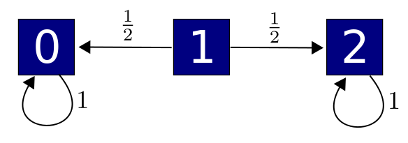
where we haven't drawn arrows labelled by 0. So, state 1 has a 50% chance of hopping to state 0 and a 50% chance of hopping to state 2; the other two states just sit there. Now, consider the observable $O$ with

$$O_i = i$$

It's easy to check that the expected value of this observable doesn't change with time:

$$ \int O U \psi = \int O \psi $$

for all $\psi$. The reason, in plain English, is this. Nothing at all happens if you start at states 0 or 2: you just sit there, so the expected value of $O$ doesn't change. If you start at state 1, the observable equals 1. You then have a 50% chance of going to a state where the observable equals 0 and a 50% chance of going to a state where it equals 2, so its expected value doesn't change: it still equals 1.

On the other hand, we do not have $[O,U] = 0$ in this example, because we can hop between states where $O$ takes different values. Furthermore,

$$ \int O^2 U \psi \ne \int O^2 \psi $$

After all, if you start at state 1, $O^2$ equals 1 there. You then have a 50% chance of going to a state where $O^2$ equals 0 and a 50% chance of going to a state where it equals 4, so its expected value changes!

So, that's why $\int O U \psi = \int O \psi $ for all $\psi$ is not enough to guarantee $[O,U] = 0$. The same sort of counterexample works for Markov processes, too.

Finally, we should add that there's nothing terribly sacred about the square of the observable. For example, we have:

Theorem. Suppose $H$ is an infinitesimal stochastic operator and $O$ is an observable. Then $$ [O,H] =0 $$

if and only if

$$ \frac{d}{d t} \int f(O) \psi(t) = 0 $$

for all smooth $f: \mathbb{R} \to \mathbb{R}$ and all $\psi(t)$ obeying the master equation.

Theorem. Suppose $U$ is a stochastic operator and $O$ is an observable. Then $$ [O,U] =0 $$

if and only if

$$ \int f(O) U \psi = \int f(O) \psi $$

for all smooth $f: \mathbb{R} \to \mathbb{R}$ and all stochastic states $\psi$

These make the 'forward direction' of Noether's theorem stronger... and in fact, the forward direction, while easier, is probably more useful! However, if we ever use Noether's theorem in the 'reverse direction', it might be easier to check a condition involving only $O$ and its square.

You can also read comments on Azimuth, and make your own comments or ask questions there!

Here's the answer to the puzzle:

Puzzle. Suppose $U$ is a stochastic operator and $O$ is an observable. Show that $O$ commutes with $U$ iff the expected values of $O$ and its square don't change when we evolve our state one time step using $U$. In other words, show that $$ [O,U] =0 $$

if and only if

and

for all stochastic states $\psi.$

Answer. One direction is easy: if $[O,U] = 0$ then $[O^n,U] = 0$ for all $ n$, so

where in the last step we use the fact that $U$ is stochastic.

For the converse we can use the same tricks that worked for Markov processes. Assume that

and

for all stochastic states $ \psi$. These imply that

and

We wish to show that $[O,U]= 0$. Note that

To show this is always zero, we'll show that when $ U_{i j} \ne 0$, then $ O_j = O_i$. This says that when our system can hop from one state to another, the observable $ O$ must take the same value on these two states.

For this, in turn, it's enough to show that the following sum vanishes for any $ j \in X$:

Why? The matrix elements $ U_{i j}$ are nonnegative since $ U$ is stochastic. Thus the sum can only vanish if each term vanishes, meaning that $ O_j = O_i$ whenever $ U_{i j} \ne 0$.

To show the sum vanishes, let's expand it:

Now, since (1) and (2) hold for all stochastic states $ \psi$, this equals

$$ \displaystyle{ O_j^2\sum_i U_{i j} - 2O_j^2 + O_j^2 } $$

But this is zero because $ U$ is stochastic, which implies

So, we're done!

© 2011 John Baez
baez@math.removethis.ucr.andthis.edu
home