


|
|
|
|
Sorry for the long pause! I've been busy writing. For example: a gentle introduction to category theory, focusing on its role as a "Rosetta Stone" that helps us translate between four languages:
1) John Baez and Mike Stay, Physics, topology, logic and computation: a Rosetta Stone, to appear in New Structures in Physics, ed. Bob Coecke. Available at http://math.ucr.edu/home/baez/rosetta.pdf
The idea is to take this chart and make it really precise:
       PHYSICS        TOPOLOGY    LOGIC        COMPUTATION
       Hilbert space  manifold    proposition  data type
       operator       cobordism   proof        program
In each case we have a kind of "thing" and a kind of "process" going between things. But it turns out we can make the analogies much sharper and more detailed than that.
The hard work has already been done by many researchers. People working on topological quantum field theory have seen how cobordisms - spacetimes going from one slice of space to another - are analogous to operators between Hilbert spaces. The "Curry-Howard correspondence" makes the analogy between proofs and programs precise. Girard's work on "linear logic" sets up an analogy between operators and proofs. And so on....
We're just trying to present these analogies in an easy-to-read form, all in one place. I hope that pondering them will help us break down some walls separating disciplines. In more optimistic moments, I even thnk they represent the first steps toward a general theory of systems and processes! Then I remember that scientists are trained to distrust such grand visions, and for good reasons. Time will tell.
But enough of that. This Week will be an ode to the number 3.
First, though... here's the nebula of the week!
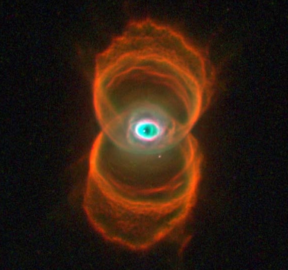
2) Hubble finds an hourglass nebula around a dying star, http://hubblesite.org/newscenter/archive/releases/nebula/planetary/1996/07/
It looks like the eye of Sauron in Tolkien's Lord of the Rings trilogy. It's not. It's a planetary nebula 8000 light years away, called MyCn 18 - or, more romantically, the Engraved Hourglass Nebula.
The colors look unreal. They are.
Okay, so the colors are fake. But how did this weird nebula form? You can see a clue if you pay attention: the bright white dwarf star isn't located exactly at the center. It's a bit to the left! This paper, written by the folks who took the photograph, argues that it has an unseen companion:
3) Raghvendra Sahai et al, The Etched Hourglass Nebula MyCn 18. I: Hubble space telescope observations, The Astronomical Journal 118 (1999), 468-476. Also available at http://www.iop.org/EJ/article/1538-3881/118/1/468/990080.text.html
This paper tackles the difficult problem of modelling the nebula:
4) Raghvendra Sahai et al, The Etched Hourglass Nebula MyCn 18. II: A spatio-kinematic model, The Astronomical Journal 110 (2000), 315-322. Also available at http://www.iop.org/EJ/article/1538-3881/119/1/315/990248.text.html
It doesn't seem that the white dwarf alone could have produced all the glowing gas we see here. A red giant companion could help. But, there are lots of mysteries.
That shouldn't be surprising. Even the simplest things can be quite rich in complexity if you look at them hard enough. I'll illustrate this with a little ode to the number 3. I'll start off slow, and ramp up to a discussion of how all these mathematical entities are locked in a tight embrace:
As I kind of intermezzo, I'll talk about how to solve the cubic equation. We all learn about quadratic equations in school: they're the bread and butter of algebra, right after linear equations. Cubics are trickier, but studying them can give you a lifetime's worth of fun.
Let's start with the trefoil knot. This is the simplest of knots:

5) Center for the Popularisation of Mathematics, Torus knots, http://www.popmath.org.uk/sculpmath/pagesm/torus2.html
Mathematically, the surface of a doughnut is called a "torus". We can describe a point on the torus by two angles running from 0 to 2π - the "latitude" and "longitude". But another name for such an angle is a "point on the unit circle". If we think of the unit circle in the complex plane, this gives us a nice equation for the trefoil:
u2 = v3
Here u and v are complex numbers with absolute value 1. The equation says that as u moves around the unit circle, v moves around 2/3 as fast. So, the set of solutions is a curve on the torus that winds around thrice in one direction while it winds around twice in the other direction - a trefoil knot!
We can also drop the restriction that u and v have absolute value 1. Then the equation u2 = v3 is famous for other reasons - it's related to cubic equations!
As you've probably heard, there's a formula for solving cubic equations, sort of like the quadratic formula, but bigger and badder. It goes back to some Italians in the 1500s who liked to challenge each other with equations and make bets on who could solve them: Scipione del Ferro, Niccolo Tartaglia and Gerolamo Cardano.
Imagine we're trying to solve a cubic equation. We can always divide by the coefficient of the cubic term, so it's enough to consider equations like this:
z3 + Az2 + Bz + C = 0
If we could solve this and find the roots a, b, and c, we could write it as:
(z - a)(z - b)(z - c) = 0
But this means
A = -(a + b + c)
B = ab + bc + ca
C = -abc
Note that A, B, and C don't change when we permute a, b, and c. So, they're called "symmetric polynomials" in the variables a, b, and c.
You see this directly, but there's also a better explanation: the coefficients of a polynomial depend on its roots, but they don't change when we permute the roots.
I can't resist mentioning a cool fact, which is deeply related to the trefoil: every symmetric polynomial of a, b, and c can be written as a polynomial in A, B, and C - and in a unique way!
In fact, this sort of thing works not just for cubics, but for polynomials of any degree. Take a general polynomial of degree n and write the coefficients as functions of the roots. Then these functions are symmetric polynomials, and every symmetric polynomial in n variables can be written as a polynomial of these - and in a unique way.
But, back to our cubic. Note that -A/3 is the average of the three roots. So, if we slide z over like this:
x = z + A/3
we get a new cubic equation for which the average of the three roots is zero. This new cubic equation will be of this form:
x3 + Bx + C = 0
for some new numbers B and C. In other words, the "A" in this new cubic is zero, since we translated the roots to make their average zero.
So, to solve cubic equations, it's enough to solve cubics like x3 + Bx + C = 0. This is a great simplification. When you first see it, it's really exciting. But then you realize you have no idea what to do next! This must be why it's called a "depressed cubic".
In fact, Scipione del Ferro figured out how to solve the "depressed cubic" shortly after 1500. So, you might think he could solve any cubic. But, negative numbers hadn't been invented yet. This prevented him from reducing any cubic to a depressed one!
It's sort of hilarious that Ferro was solving cubic equations before negative numbers were worked out. It should serve as a lesson: we mathematicians often work on fancy stuff before understanding the basics. Often that's why math seemss hard! But often it's impossible to discover the basics except by working on fancy stuff and getting stuck.
Here's one trick for solving the depressed cubic x3 + Bx + C = 0. Write
x = y - B/(3y)
Plugging this in the cubic, you'll get a quadratic equation in y3, which you can solve. From this you can figure out y, and then x.
Alas, I have no idea what this trick means. Does anyone know? Ferro and Tartaglia used a more long-winded method that seems just as sneaky. Later Lagrange solved the cubic yet another way. I like his way because it contains strong hints of Galois theory.
You can see all these methods here:
6) Wikipedia, Cubic function, http://en.wikipedia.org/wiki/Cubic_equation.
So, I won't say more about solving the cubic now. Instead, I want to explain the "discriminant". This is a trick for telling when two roots of our cubic are equal. It turns out to be related to the trefoil knot.
For a quadratic equation ax2 + bx + c = 0, the two roots are equal precisely when b2 - 4ac = 0. That's why b2 - 4ac is called the "discriminant" of the quadratic. The same idea works for other equations; let's see how it goes for the cubic.
Suppose we were smart enough to find the roots of our cubic
x3 + Bx + C = 0
and write it as
(x - a)(x - b)(x - c) = 0
Then two roots are equal precisely when
(a - b)(b - c)(c - a) = 0
The left side isn't a symmetric polynomial in a, b, and c; it changes sign whenever we switch two of these variables. But if we square it, we get a symmetric polynomial that does the same job:
D = (a - b)2 (b - c)2 (c - a)2
This is the discriminant of the cubic! By what I said about symmetric polynomials, it has to be a polynomial in B and C (since A = 0). If you sweat a while, you'll see
D = -4B3 - 27C2
So, here's the grand picture: we've got a 2-dimensional space of cubics with coordinates B and C. Sitting inside this 2d space is a curve consisting of "degenerate" cubics - cubics with two roots the same. This curve is called the "discriminant locus", since it's where the discriminant vanishes:
4B3 + 27C2 = 0
If we only consider the case where B and C are real, the discriminant locus looks like this:
                   |C
           o       |
            o      |
               o   |
        -----------o-------------
               o   |           B
            o      |
           o       |
                   |
It's smooth except at the origin, where it has a sharp point called
a "cusp".
Now here's where the trefoil knot comes in. The equation for the discriminant locus:
4B3 + 27C2 = 0
should remind you of the equation for the trefoil:
u2 = v3
Indeed, after a linear change of variables they're the same! But, for the trefoil we need u and v to be complex numbers. We took them to be unit complex numbers, in fact.
So, the story is this: we've got a 2-dimensional complex space of complex cubics. Sitting inside it is a complex curve, the discriminant locus. In our new variables, it's this:
u2 = v3
If we intersect this discriminant locus with the torus
|u| = |v| = 1
we get a trefoil knot. But that's not all!
Normal folks think of knots as living in ordinary 3d space, but topologists often think of them as living in a 3-sphere: a sphere in 4d space. That's good for us. We can take this 4d space to be our 2d complex space of complex cubics! We can pick out spheres in this space by equations like this:
|u|2 + |v|3 = c (c > 0)
These are not round 3-spheres, thanks to that annoying third power. But, they're topologically 3-spheres. If we take any one of them and intersect it with our discriminant locus, we get a trefoil knot! This is clear when c = 2, since then we have
|u|2 + |v|3 = 2
and
u2 = v3
which together imply
|u| = |v| = 1
But if you think about it, we also get a trefoil knot for any other c > 0. This trefoil shrinks as c → 0, and at c = 0 it reduces to a single point, which is also the cusp here:
                     |u
                     |      o
                     |     o
                     |   o
          -----------o-------------
                     |   o        v
                     |     o
                     |      o
                     |
We don't see trefoil knots in this picture because it's just a
real 2d slice of the complex 2d picture. But, they're lurking in
the background!
Now let me say how the group of permutations of three things gets into the game. We've already seen the three things: they're the roots a, b, and c of our depressed cubic! So, they're three points on the complex plane that add to zero. Being a physicist at heart, I sometimes imagine them as three equal-mass planets, whose center of mass is at the origin.
The space of possible positions of these planets is a 2d complex vector space, since we can use any two of their positions as coordinates and define the third using the relation
a + b + c = 0
So, there are three coordinate systems we can use: the (a,b) system, the (b,c) system and the (c,a) system. We can draw all three coordinate systems at once like this:
                b
                 \       /
                  \     /
                   \   /
                    \ /
             --------o--------a
                    / \
                   /   \
                  /     \
                 /       \
                c
The group of permutations of 3 things acts on this picture
by permuting the three axes. Beware: I've only drawn a 2-dimensional
real vector space here, just a slice of the full 2d complex space.
Now suppose we take this 2d complex space and mod out by the permutation symmetries. What do we get? It turns out we get another 2d complex vector space! In this new space, the three coordinate axes shown above become just one thing... but this thing is a curve, like this:
            o
             o
                o
                   o
                o
             o
            o
Look familiar? Sure! It's just the discriminant locus we've
seen before.
Why does it work this way? The explanation is sitting before us. We've got two 2d complex vector spaces: the space of possible ordered triples of roots of a depressed cubic, and the space of possible coefficients. There's a map from the first space to the second, since the coefficients are functions of the roots:
B = ab + bc + ca
C = -abc
These functions are symmetric polynomials: they don't change when we permute a, b, and c. And, it follows from what I said earlier that we can get any symmetric polynomial as a function of these - under the assumption that a+b+c = 0, that is.
So, the map where we mod out by permutation symmetries of the roots is exactly the map from roots to coefficients.
The lines in this picture are places where two roots are equal:
            c=a
              \       /
               \     /
                \   /
                 \ /
          --------o-------- b=c
                 / \
                /   \
               /     \
              /       \
            a=b
So, when we apply the map from roots to coefficients, these lines
get mapped to the discriminant locus:
                  |
          o       |
           o      |
              o   |
       -----------o-------------
              o   |
           o      |
          o       |
                  |
You should now feel happy and quit reading... unless you
know a bit of topology. If you do know a little topology,
here's a nice spinoff of what we've done. Though I didn't say
it using so much jargon, we've already seen that space of
nondegenerate depressed cubics is C2 minus a cone on the
trefoil knot. So, the fundamental group of this space is the
same as the fundamental group of S3 minus a trefoil knot.
This is a famous group: it has three generators x,y,z, and three
relations saying that:
On the other hand, we've seen this space is the space of triples of distinct points in the plane, centered at the origin, mod permutations. The condition "centered at the origin" doesn't affect the fundamental group. So, this fundamental group is another famous group: the "braid group on 3 strands". This has two generators:
\ /  |
 /   |          X
/ \  |
and
|  \ /
|   /           Y
|  / \
and one relation, called the "Yang-Baxter equation" or "third Reidemeister move":
\ /  |        |  \ /
 /   |        |   /
/ \  |        |  / \
|  \ /        \ /   |
|   /     =    /    |           XYX = YXY
|  / \        / \   |
\ /  |        |  \ /
 /   |        |   /
/ \  |        |  / \
So: the 3-strand braid group is isomorphic to the fundamental group of the complement of the trefoil! You may enjoy checking this algebraically, using generators and relations, and then figuring out how this algebraic proof relates to the geometrical proof.
I find all this stuff very pretty...
... but what's really magnificent is that most of it generalizes to any Dynkin diagram, or even any Coxeter diagram! (See "week62" for those.)
Yes, we've secretly been studying the Coxeter diagram A2, whose "Coxeter group" is the group of permutations of 3 things, and whose "Weyl chambers" look like this:
                 \       /
                  \     /
                   \   /
                    \ /
             --------o--------
                    / \
                   /   \
                  /     \
                 /       \
Let me just sketch how we can generalize this to An-1. Here
the Coxeter group is the group of permutations of n things, which
I'll call n!.
Let X be the space of n-tuples of complex numbers summing to 0. X is a complex vector space of dimension n-1. We can think of any point in X as the ordered n-tuple of roots of some depressed polynomial of degree n. Here "depressed" means that the leading coefficient is 1 and the sum of the roots is zero. This condition makes polynomials sad.
The permutation group n! acts on X in an obvious way. The quotient X/n! is isomorphic (as a variety) to another complex vector space of dimension n-1: namely, the space of depressed polynomials of degree n. The quotient map
X → X/n!
is just the map from roots to coefficients!
Sitting inside X is the set D consisting of n-tuples of roots where two or more roots are equal. D is the union of a bunch of hyperplanes, as we saw in our example:
                  \       /
                   \     /
                    \   /
                     \ /
              --------o--------
                     / \
                    /   \
                   /     \
                  /       \
Sitting inside X/n! is the "discriminant locus" D/n!, consisting
of degenerate depressed polynomials of degree n - that is, those
with two or more roots equal. This is a variety that's smooth except for
some sort of "cusp" at the origin:
              o
               o
                  o
                      o
                  o
               o
              o
The fundamental group of the complement of the discriminant locus
is the braid group on n strands. The reason is that this group
describes homotopy classes of ways that n points in the plane can
move around and come back to where they were (but possibly permuted).
These points are the roots of our polynomial.
On the other hand, the discriminant locus is topologically the cone on some higher-dimensional knot sitting inside the unit sphere in Cn-1. So, the fundamental group of the complement of this knot is the braid group on n strands.
This relation between higher-dimensional knots and singularities was investigated by Milnor, not just for the An series of Coxeter diagrams but more generally:
7) John W. Milnor, Singular Points of Complex Hypersurfaces, Princeton U. Press, 1969.
The other Coxeter diagrams give generalizations of braid groups called Artin-Brieskorn groups. Algebraically you get them by taking the usual presentations of the Coxeter groups and dropping the relations saying the generators (reflections) square to 1.
If you like braid groups and Dynkin diagrams, Artin-Brieskorn groups are irresistible! For a fun modern account, try:
8) Daniel Allcock, Braid pictures for Artin groups, available as arXiv:math.GT/9907194.
But I'm digressing! I must return and finish my ode to the number 3. I need to say how modular forms get into the game!
I'll pick up the pace a bit now - if you're tired, quit here.
Any cubic polynomial P(x) gives something called an "elliptic curve". This consists of all the complex solutions of
y2 = P(x)
together with the point (∞, ∞), which we include to make things nicer.
Clearly this elliptic curve has two points (x,y) for each value of x except for x = ∞ and the roots of P(x), where it just has one. So, it's a "branched double cover" of the Riemann sphere, with branch points at the roots of our cubic and the point at infinity.
In fact, this elliptic curve has the topology of a torus, at least when all the roots of our cubic are different. If you have trouble imagining a torus that's a branched double cover of a sphere, ponder this:
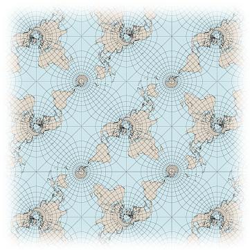
9) Carlos Furuti, Peirce's quincuncial map, http://www.progonos.com/furuti/MapProj/Normal/ProjConf/projConf.html
This square map of the Earth is an unwrapped torus; each point of the Earth shows up lots of times. If we wrap it up just right, we get a branched double cover of the sphere! Can you spot the branch points? For a lot more explanation, read "week229".
Now, way back in "week13", I turned this story around. I started with a torus formed as the quotient of the complex plane by a lattice - and showed how to get an elliptic curve out of it. I wrote the equation for this elliptic curve in "Weierstrass form":
y2 = 4x3 - g2 x - g3
By a simple change of variables, this is equivalent to a depressed cubic:
y2 = x3 + Bx + C
So, we can think of g2 and g3 as coordinates on our 2d space of depressed cubics! They're just rescaled versions of our coordinate functions B and C.
What's the big deal? Well, g2 and g3 are famous examples of "modular forms" - whatever those are. In fact, it's a famous fact that every modular form is a polynomial in g2 and g3.
I defined modular forms back in "week142", where I summarized the Taniyama-Shimura-Weil theorem: the big theorem about modular forms that implies Fermat's Last Theorem. So, you can reread the definition there if you're curious. But if you've never seen it before, it's a bit intimidating. A modular form of weight w is a function on the space of lattices that transforms in a certain bizarre way, satisfying a certain growth condition... blah blah blah.
It's important stuff, and incredibly cool once you get a feel for it. But suppose we're trying to explain modular forms more simply. Then we can avoid a lot of technicalities if we just say a modular form is a polynomial on the space of depressed cubics! In other words, a polynomial in our friends B and C.
Then we can make some definitions. The "weight" of the modular form
Bi Cj
is 4i+6j. Okay, I admit this sounds arbitrary and weird without a lot more explanation. But better: a "cusp form" is a modular form that vanishes on the discriminant locus. Then we can see every cusp form is the product of the discriminant 4B3 + 27C2 and some other modular form... and we can use this to work out lots of basic stuff about modular forms.
So, I hope you now see how tightly entwined all these ideas are:
At this point I should give credit where credit is due. As usual, I've been talking to Jim Dolan, and many of these ideas come from him. But also, you can think of this Week as an expansion of the remarks by Joe Christy and Swiatowslaw Gal in the Addenda to "week233". And, it was Chris Hillman who first told Jim and me that SL(2,R)/SL(2,Z) looks like S3 minus a trefoil knot.
Finally, I should say that my low-budget approach to modular forms mostly just handles so-called "level 0" modular forms - the basic kind, defined using the group
Γ = PSL(2,Z)
More exciting are modular forms that transform nicely only for a subgroup of Γ. Jim and I are just beginning to understand these. But the modular forms for Γ(2) fit nicely into today's ode! Here Γ(2) is the subgroup of Γ consisting of matrices congruent to the identity matrix mod 2. What does this have to do with my ode to the number 3? Well,
Γ/Γ(2) ≅ PSL(2,F2)
and this is isomorphic to the group of permutations of 3 things!
So, as a final flourish, I claim that:
Modular forms for Γ(2) are polynomials on the space X consisting of roots of depressed cubics:
X = {(a,b,c): a,b,c complex with a + b + c = 0}
Modular forms for Γ are polynomials on the space X/3! consisting of coefficients of depressed cubics:
X/3! = {(B,C): B,C complex}
The obvious quotient map X → X/3! sends roots to coeffficients:
(a,b,c) |→ (B,C) = (ab + bc + ca, abc)
and this induces the inclusion of modular forms for Γ into modular forms for Γ(2):
B |→ ab + bc + ca
C |→ abc
I hope this is all true!
Modular forms for Γ(2) are particularly nice. A good example is the cross-ratio, much beloved in complex analysis. If you want to learn more about this stuff, try:
10) Igor V. Dolgachev, Lectures on modular forms, Fall 1997/8, available at http://www.math.lsa.umich.edu/~idolga/modular.pdf
especially chapter 9 for level 2 modular forms. Also:
11) Henry McKean and Victor Moll, Elliptic Curves: Function Theory, Geometry, Arithmetic, Cambridge U. Press, 1999.
especially chapter 4.
Addendum: For more discussion, go to the n-Category Café.
© 2008 John Baez
baez@math.removethis.ucr.andthis.edu
|
|
|
|