December 19, 2009

This Week's Finds in Mathematical Physics (Week 287)

John Baez

This week: a fascinating history of categorical logic, and more about rational homotopy theory. But first, guess what this is a picture of:

If you give up, go to the bottom of this article.

Next, here's an incredibly readable introduction to the revolution that happened in logic starting in the 1960s:

1) Jean-Pierre Marquis and Gonzalo Reyes, The history of categorical logic, 1963-1977. Available at https://www.webdepot.umontreal.ca/Usagers/marquisj/MonDepotPublic/HistofCatLog.pdf

It's a meaty but still bite-sized 116 pages. It starts with the definitions of categories, functors, and adjoint functors. But it really takes off in 1963 with Bill Lawvere's thesis, which revolutionized universal algebra using category theory. It then moves on through Lawvere and Tierney's introduction of the modern concept of topos, and it ends in 1977, when Makkai and Reyes published their book on categorical logic, and Johnstone published his book on topos theory. The world has never been the same since!

One great thing about this paper is that it discusses the history in a blow-by-blow way, including conferences and unpublished but influential writings. It also gives a great summary of the key ideas in Lawvere's thesis. I'll quote it, since everyone should know or at least have seen these ideas:

1. To use the category of categories as a framework for mathematics, i.e. the category of categories should be the foundations of mathematics;

2. Every aspect of mathematics should be representable in one way or another in that framework; in other words, categories constitute the background to mathematical thinking in the sense that, in this framework, essential features of that thinking are revealed;

3. Mathematical objects and mathematical constructions should be thought of as functors in that framework;

4. In particular, sets always appear in a category, there are no such thing as sets by themselves, in fact there is no such thing as a mathematical concept by itself;

5. But sets form categories and the latter categories play a key role in the category of categories, i.e. in mathematics;

6. Adjoint functors occupy a key position in mathematics and in the development of mathematics; one of the guiding principles of the development of mathematics should be "look for adjoints to given functors"; in that way foundational studies are directly linked to mathematical practice and the distinction between foundational studies and mathematical studies is a matter of degree and direction, it is not a qualitative distinction;

7. As the foregoing quote clearly indicates, Lawvere is going back to the claim made by Eilenberg and Mac Lane that the "invariant character of a mathematical discipline can be formulated in these terms" [i.e. in terms of functoriality]. But now, in order to reveal this invariant character, extensive use of adjoint functors is made.

8. The invariant content of a mathematical theory is the "objective" content of that theory; this is expressed at various moments throughout his publications. To wit:

As posets often need to be deepened to categories to accurately reflect the content of thought, so should inverses, in the sense of group theory, often be replaced by adjoints. Adjoints retain the virtue of being uniquely determined reversal attempts, and very often exist when inverses do not.

9. Not only sets should be treated in a categorical framework, but also logical aspects of the foundations of mathematics should be treated categorically, in as much as they have an objective content. In particular, the logical and the foundational are directly revealed by adjoint functors.

If this sounds mysterious, well, read the paper!

Now I want to dig a little deeper into rational homotopy theory, and start explaining this chart:

                      RATIONAL SPACES
                         /      \  
                        /        \  
                       /          \  
                      /            \
                     /              \
      DIFFERENTIAL GRADED ------- DIFFERENTIAL GRADED
      COMMUTATIVE ALGEBRAS           LIE ALGEBRAS
      

That's what the other corners of this triangle are. The lower left corner involves a drastic generalization of differential forms on smooth manifolds. The lower right corner involves a drastic generalization of Lie algebras coming from Lie groups.

Today I'll explain the road to the lower left corner. Very roughly, it goes like this. If you give me a space, I can replace it with a space made of simplices that has the same homotopy type, and then take the differential forms on this replacement. Voilà! A differential graded commutative algebra!

But I want to avoid talking to just the experts. Among other things, I want to use rational homotopy theory as an excuse to explain lots of good basic math. So, first I'll remind you about differential forms on a manifold, and why they're a "differential graded commutative algebra", or "DGCA" for short. Then I'll show you how to define something like differential forms starting from any topological space! Again, they're a DGCA. And it turns out that for rational spaces, this DGCA knows everything there is to know about our space - at least as far as homotopy theory is concerned.

So: what are differential forms? Differential forms are a basic tool for doing calculus on manifolds. We use them throughout physics: they're the grownup version of the "gradient", "divergence" and "curl" that we learn about as kids. There are lots of ways to define them, but the most rapid is this.

The smooth real-valued functions

f: X → R

on a manifold X form an algebra over the real numbers. In other words: you can add and multiply them, and multiply them by real numbers, and a bunch of familiar identities hold, which are the axioms for an algebra. Moreover, this algebra is commutative:

fg = gf

Starting from this commutative algebra, or any commutative algebra A, we can define differential forms as follows. First let's define vector fields in a purely algebraic way. Since the job of a vector field is to differentiate functions, people call them derivations in this algebraic approach. A "derivation of A" is a linear map

v: A → A

which obeys the product rule

v(ab) = v(a)b + av(b)

Let Der(A) be the set of derivations of A. This is a "module" of the algebra A, since we can multiply a derivation by a guy in A and get a new derivation. (This part works only because A is commutative.)

Next let's define 1-forms. Since the job of these is to eat vector fields and spit out functions, let's define a "1-form" to be a linear map

ω: Der(A) → A

which is actually a module homomorphism, meaning

ω(fv) = f ω(v)

whenever f is in A. Let Ω¹(A) be the set of 1-forms. Again, this is a module of A.

Just as you'd expect, there's a map

d: A → Ω¹(A)

defined by

(df)(v) = v(f)

and you can check that

d(fg) = (df) g + f dg

So, we've got vector fields and 1-forms! It's a bit tricky, but you can prove that when A is the algebra of smooth real-valued functions on a manifold, the definitions I just gave are equivalent to all the usual ways of defining vector fields and 1-forms. One advantage of working algebraically is that we can generalize. For example, we can take A to consist of polynomial functions. We'll use this feature in a minute.

But what about other differential forms? There's more to life than 1-forms: there are p-forms for p = 0,1,2,...

To get these, we just form the exterior algebra of the module Ω¹(A). You may have seen the exterior algebra of a vector space - if not, it may be hard understanding the stuff I'm explaining now. The exterior algebra of a module over a commutative algebra works the same way! To build it, we run around adding and multiplying guys in A and Ω¹(A), all the while making sure to impose the axioms of an associative unital algebra, together with these rules:

f (dg) = (dg) f

(df) (dg) = - (dg) (df)

The stuff we get forms an algebra: the algebra of "differential forms" for A, which I'll call Ω(A). And when A is the smooth functions on a manifold, these are the usual differential forms that everyone talks about!

Now, thanks to the funny rule

(df) (dg) = - (dg) (df)

the algebra Ω(A) is not commutative. However, it's "graded commutative", meaning roughly that it's commutative except for some systematically chosen minus signs.

A bit more precisely: every differential form can be written as a linear combination of guys like this:

v = f dg₁ dg₂ … dg_p

where p ranges over all natural numbers. Linear combinations of guys of this sort for a particular fixed p are called "p-forms". We also say they're "of degree p". And the algebra of differential forms obeys

νω = (-1)^pq ων

whenever ν is of degree p and ω is of degree q. This is what we mean by saying Ω(A) is "graded commutative".

But the algebra of differential forms is better than a mere graded commutative algebra! We've already introduced df when f is an element of our original algebra. But we can define "d" for all differential forms simply by saying that d is linear and saying that d of

f dg₁ dg₂ ... dg_p

is

df dg₁ dg₂ ... dg_p

This definition implies three facts. First, it implies that d of a p-form is a (p+1)-form. That's pretty obvious. Second, it implies that

d(dω) = 0

for any differential form ω. Why? Well, I'll let you check it, but I'll give you a hint: the key step is to show that d1 = 0. And third, it implies this version of the product rule:

d(νω) = (dν) ω + (-1)^p νdω

for any p-form ν and q-form ω. Again the proof is a little calculation.

We can summarize these three facts, together with the linearity of d, by saying that differential forms are a "differential graded commutative algebra", or "DGCA".

You can do lots of wonderful stuff with differential forms. After you learn a bunch of this stuff, it becomes obvious that you should generalize them to apply to spaces of many kinds.

It's easy to generalize them from manifolds to spaces X where you have a reasonable idea of when a real-valued function

f: X → R

counts as "smooth". Just take the commutative algebra A of smooth real-valued functions on X and construct Ω(A) following my instructions!

There are many examples of such spaces, including manifolds with boundary, manifolds with corners, and infinite-dimensional manifolds. In fact, there are general theories of "smooth spaces" that systematically handle lots of these examples:

2) Andrew Stacey, Comparative smootheology, available as arXiv:0802.2225.

3) Patrick Iglesias-Zemmour, Diffeology. Available at http://math.huji.ac.il/~piz/Site/The%20Book/The%20Book.html

4) John Baez and Alexander Hoffnung, Convenient categories of smooth spaces, to appear in Trans. Amer. Math. Soc.. Also available as arXiv:0807.1704.

But here's a question that sounds harder: how can we generalize differential forms to an arbitrary topological space X?

You could take A to be the algebra of continuous functions on X and form Ω(A). There's no law against it... go ahead... but I bet no good will come of it. (What goes wrong?)

But there's a better approach, invented by Dennis Sullivan in this famous paper:

5) Dennis Sullivan, Infinitesimal computations in topology, Publications Mathimatiques de l'IHES 47 (1977), 269-331. Available at http://www.numdam.org/item?id=PMIHES_1977__47__269_0

We start by turning our topological space into a simplicial set. Remember, a simplicial set is a bunch of

0-simplices (vertices)
1-simplices (edges)
2-simplices (triangles)
3-simplices (tetrahedra)

and so on, all stuck together. Given a topological space X, we can form an enormous simplicial set whose n-simplices are all possible maps

f: Δⁿ → X

where Δⁿ is the standard n-simplex, that is, the intersection of the hyperplane

x₀ + x₁ + ... + x_n = 1

with the set where all the coordinates x_i are nonnegative.

This enormous simplicial set is called the "singular nerve" of X, Sing(X). Like any simplicial set, we can think of Sing(X) as a purely combinatorial gadget, but we can also "geometrically realize" it and think of it as a topological space in its own right. The resulting space is called |Sing(X)|.

(For more details on the singular nerve and its geometric realization, see items E and F of "week116".)

This space |Sing(X)| is made of a bunch of simplices stuck together along their faces. So, we can say a real-valued function on |Sing(X)| is "simplex-wise smooth" if it's continuous and smooth on each simplex. And this is enough to set up a theory of differential forms! We just take the algebra A of simplex-wise smooth functions on |Sing(X)|, and use this to build our algebra of differential forms Ω(A) as I've described!

But Sullivan noted that we can go even further. Thanks to how we've defined the standard n-simplex, it makes sense to talk about polynomial functions on this simplex. We can even sidestep the need for real numbers, by looking at polynomial functions with rational coefficients. And that's just right for rational homotopy theory.

So, let's focus our attention on functions on |Sing(X)| that when restricted to any simplex give polynomials with rational coefficients. This is a commutative algebra over the rational numbers. Call it A. We can copy our previous construction of Ω(A) but now working with rational numbers instead of reals. Let's call guys in here "rational differential forms".

Now, you may complain that we're not really studying differential forms on X: we're studying them on this other space |Sing(X)|. At one point in my life this really annoyed me. It seemed like a cheat. But for the purposes of homotopy theory it's perfectly fine, since |Sing(X)| has the same homotopy type as X.

(By this, I really mean they're isomorphic in the "homotopy category", which I defined last week. So: they're the same, as far as homotopy theory is concerned.)

And even better, when X is a rational space, the rational differential forms on |Sing(X)| will know everything about the homotopy type of X. This is amazing! It means that for rational spaces, we can reduce homotopy theory to a souped-up version of the theory of differential forms!

In particular, Sullivan was able to use this trick to compute the homotopy groups of a rational space X, starting from the rational differential forms on |Sing(X)|.

Since X and |Sing(X)| have the same homotopy type, they have the same homotopy groups, and cohomology groups, and so on. And it's not surprising that we can read off the cohomology groups of |Sing(X)| starting from the rational differential forms on this space - this is just a slight twist on the usual idea of deRham cohomology. But it's surprising that we can compute the homotopy groups, which are usually a lot harder. This is the magic of rational homotopy theory.

I won't explain this magic, at least not today. For that read Sullivan's paper, or this paper I recommended last time:

6) Kathryn Hess, Rational homotopy theory: a brief introduction, in Interactions Between Homotopy Theory and Algebra, ed. Luchezar L. Avramov, Contemp. Math 436, AMS, Providence, Rhode Island, 2007. Also available as math.AT/0604626.

For more detail, try this book:

7) Phillip A. Griffiths and John W. Morgan, Rational Homotopy Theory and Differential Forms, Birkhäuser, Boston, 1981.

Someday I should explain exactly the sense in which (certain) DGCAs are "the same" as rational homotopy types. But not today!

Instead, I want to go over what I just said in a slightly more formal way. This will give me an excuse to introduce a bunch of beautiful concepts that everyone should know... and maybe demonstrate a tiny bit of what Lawvere was talking about: the power of categories.

First of all, what's a DGCA, really? It's a commutative monoid in the symmetric monoidal category of cochain complexes!

Let me explain.

A "cochain complex", for us, will be a list of vector spaces and linear maps

    d       d      d
C0 ---> C1 ---> C2 ---> ...

Just as you can tensor vector spaces, you can tensor cochain complexes. The tensor product of cochain complexes C and C' will have

(C ⊗ C')_n = &oplus_{p+q = n} C_p ⊗ C'_q

and we define

d(c ⊗ c') = dc ⊗ c' + (-1)^p c ⊗ dc'

when c is in C_p and c' is in C'_q.

(You've seen a similar "product rule" earlier in this article. There's a general principle at work here. Physicists know that whenever you exchange two fermions, their phase gets multiplied by -1. In math, we should stick in a minus sign whenever we switch two "odd" things. The map d counts as odd since it sends guys in our cochain complex to guys whose degree is 1 more, and the number 1 is odd. The element c in C_p counts as "odd" whenever p is odd. In the equation above, we're switching d past c and getting a minus sign whenever c is odd.)

Just as you can define a commutative algebra to be a vector space V with a product

V ⊗ V → V

that's associative and commutative, you can define a "differential graded commutative algebra", or DGCA, to be a cochain complex C with a product

C ⊗ C → C

that's associative and graded-commutative. By "graded-commutative", I mean you need to remember to put in a sign (-1)^pq whenever you switch a guy in C^p and a guy in C^q.

We can systematize all this by checking that, just like the category of vector spaces with its usual tensor product, the category of cochain complexes with its tensor product is a "symmetric monoidal category":

8) nLab, Symmetric monoidal category, http://ncatlab.org/nlab/show/symmetric+monoidal+category

So is the category of sets with its cartesian product. We can define a "commutative monoid" in any symmetric monoidal category. In the category of sets, this is just a commutative monoid in the traditional sense. In the category of vector spaces, it's a commutative algebra. And in the category of cochain complexes, it's a DGCA!

Notice: a DGCA where only C₀ is nonzero is just a plain old commutative algebra. So, DGCAs really are a generalization of commutative algebras. So whenever anyone tells you something about DGCAs, you should check to see what it says about commutative algebras. And whenever anyone tells you something about commutative algebras, you should try to generalize it to DGCAs!

This should keep you pretty busy, since commutative algebras are the playground of the simplest kind of algebraic geometry: the kind where you look at solutions of polynomial equations in a bunch of variables, like this:

x² + y² + z² = 0
xyz - 1 = 0

If you take your polynomials and count them as zero when they satisfy your equations, you get a commutative algebra. Even better, you can get any sufficiently small commutative algebra this way - the technical term is "finitely presented". And if you allow infinitely many variables and infinitely many equations, you can drop that technical fine print.

So, the study of commutative algebras is really just the study of polynomial equations. And if we think about their solutions as forming curves or surfaces or the like, we're doing algebraic geometry - so-called "affine" algebraic geometry.

This means that we can - and in fact should! - generalize all of affine algebraic geometry from commutative algebras to DGCAs. I'd like to say more about this someday... but not today. This is just a digression. I got distracted from my real goal.

Before I got distracted, I was telling you how commutative algebras are the same as DGCA's with only C₀ being nonzero. And here's why I mentioned this. We can take any DGCA and violently kill C_p for all p > 0, leaving a commutative algebra C₀. We can think of this as a forgetful functor

[DGCAs] → [commutative algebras]

And this functor has a left adjoint, which freely generates a DGCA starting from a commutative algebra:

[commutative algebras] → [DGCAs]

Now, I've already told you about process that takes a commutative algebra and creates the DGCA. Namely, the process that takes a commutative algebra A and gives the DGCA of differential forms, Ω(A). So, you might think this left adjoint is just that!

I thought so too, when I was first writing this. But it turns out not to be true - at least not always! The left adjoint gives a slightly different kind of differential forms for our commutative algebra A. Let's call these the "Kähler forms" Ω_K(A).

The Kähler 1-forms are usually called "Kähler differentials". We can can build them as follows: take the A-module generated by symbols

df

which obey the 3 basic relations we expect in calculus:

d(cf) = c df

d(f + g) = df + dg

d(fg) = f dg + (df) g

where f,g are in A and c is in our field. This gives the A-module of Kähler differentials - let's call this Ω_K¹(A). The Kähler forms Ω_K(A) are then the exterior algebra on Ω_K¹(A).

By how we've set things up, the Kähler differentials are blessed with a map

d: A → Ω_K¹(A)

And this map is a "derivation", meaning it satisfies the 3 rules listed above. But here's the cool part: the Kähler differentials are the universal A-module with a derivation. In other words, suppose M is any A-module equipped with a map

v: A → M

that's a derivation in the above sense. Then there's a unique A-module homomorphism

j: Ω_K¹(A) → M

such that

v = j d

The proof is easy: just define j(df) = v(f) and check that everything works!

Thanks to this universal property, Kähler differentials are much beloved by algebraists. So, it's natural to wonder if they're the same as the 1-forms Ω¹(A) that I explained above!

As it turns out, these 1-forms are the double dual of the Kähler differentials:

Ω¹(A) = Ω_K¹(A)**

Sometimes we get

Ω¹(A) = Ω_K¹(A)

and this case it's easy to check that

Ω(A) = Ω_K(A)

But sometimes the 1-forms and the Kähler differentials are different. Let me explain why. It's technical, but fun if you're already familiar with some of these ideas.

For starters, let me explain what I mean! We've got a commutative algebra A. If we have an A-module M, its "dual" M* is the set of all A-module maps

w: M → A

The dual becomes a module in its own right by

(gw)(f) = g w(f)

So, we can take the dual of the dual, M**. And then there's always a module homomorphism

j: M → M**

given by

j(f)(w) = w(f)

for f in M, w in M*. Sometimes j is an isomorphism: for example, when M is finitely generated and projective. But often it's not. And that's where the subleties arise.

If you look back at my definition of 1-forms, it amounted to this:

Ω¹(A) = Der(A)*

And the universal property of Kähler differentials gives us this:

Der(A) ≅ Ω_K¹(A)*

Putting these facts together, we get

Ω¹(A) ≅ Ω_K¹(A)**

So, we always have a module homomorphism

j: Ω_K¹(A) → Ω¹(A)

This is both the map we always get from a module to its double dual, and the map we get from the universal property of Kähler differentials.

Now, here's the tricky part. This map j is always a surjection. And it will be an isomorphism when the Kähler differentials are a finitely generated projective module. But it won't always be an isomorphism!

For example, when A is the algebra of rational polynomials on a simplex, Ω_K¹(A) is a finitely generated projective module. In fact it's the free module with one generator dx_i for each independent coordinate. So in this case we actually get an isomorphism

Ω¹(A) ≅ Ω_K¹(A)

and thus

Ω(A) ≅ Ω_K(A)

More generally, this is true whenever A is the algebraic functions on a smooth affine algebraic variety, by the same sort of argument. So in these cases, you don't need to worry about the niggling nuances I'm rubbing your nose in here.

But when A is the algebra of smooth functions on a manifold, the 1-forms are not the same as the Kähler differentials!

Indeed, let A be the algebra of smooth functions on the real line. Then one can show

j: Ω_K¹(A) → Ω¹(A)

is not one-to-one. In fact, David Speyer showed this after Maarten Bergvelt noticed I was being overoptimistic in assuming otherwise. You can see Speyer's argument here:

9) David Speyer, Kahler differentials and ordinary differentials, Math Overflow, http://mathoverflow.net/questions/6074/kahler-differentials-and-ordinary-differentials/9723#9723

He shows that in Ω_K¹(A), d(e^x) is not equal to e^x dx. The intuition here is simple: showing these guys are equal requires actual calculus, with limits and stuff. But Kähler differentials are defined purely algebraically, so they don't know that stuff!

However, turning this idea into a proof takes work. It can't be as easy as I just made it sound! After all, Ω¹(A) was also defined purely algebraically, and in here we do have d(e^x) = e^x dx. Indeed, this is why Speyer's argument shows that

j: Ω_K¹(A) → Ω¹(A)

fails to be one-to-one.

So now you should be wondering: how do we know d(e^x) = e^x dx in &Omega¹(A)? Since Ω¹(A) is the dual of the derivations, to show

d(e^x) = e^x dx

we just need to check that they agree on all derivations. The hard part is to prove that any derivation of A is of the form

v(f) = g f ′

for some g in A, where f ′ is the usual derivative of f. Then we have

d(e^x)(v) = v(e^x) = g e^x = e^x v(x) = (e^x dx)(v)

so we're done!

(Here x is the usual function by that name on the real line - you know, the one that equals x at the point x. Sorry - that sounds really stupid! But anyway, the derivative of x is 1, so v(x) = g.)

So here's the hard part. Say we have a derivation v of the algebra A of smooth functions on the real line. Why is there a function g such that

v(f) = g f ′

for all functions f? As you can guess from my parenthetical remark, we should try

g = v(x)

So, let's prove

v(f) = v(x) f ′

We just need to check they're equal at any point x₀. So, let's use a kind of Taylor series trick:

f(x) = f(x₀) + (x - x₀) f ′(x₀) + (x - x₀)² h(x)

Here it's utterly crucial that h is a smooth function on the real line. Check that yourself!!! Then, apply the derivation v and use the three rules that derivations obey:

v(f)(x) = v(x) f ′(x₀) + 2(x - x₀) v(x) h(x) + (x - x₀)² v(h)

Then evaluate both sides at x = x₀. A bunch of stuff goes away:

v(f)(x₀) = v(x) f ′(x₀)

Since this was true for any point x₀, we indeed have

v(f) = v(x) f ′

as desired.

Sneaky, huh? The argument looked "purely algebraic" - but only because we could pack all the calculus into the utterly crucial bit that I made you check for yourself. By the way, this utterly crucial bit uses the theory of "Hadamard quotients": if f is smooth function on the real line then

(f(x) - f(y))/(x - y)

extends to a smooth function on the plane if we define it to be the derivative of f when x = y.

A fancier version of this argument works for Rⁿ. This in turn gives the usual proof that that derivations of the algebra A of smooth functions on a manifold X are the same as smooth vector fields. And that, in turn, guarantees that Ω(A) as defined algebraically matches the ordinary concept of differential forms on X. The Kähler forms are different, but as we've seen, there's a surjection of DGCAs

j: Ω_K(A) → Ω(A)

sending any function f in Kähler land to the same function f in ordinary differential form land.

So that's the story! It's a bit technical, but if we didn't occasionally enjoy being dragged through the mud of technical details, we wouldn't like math, now, would we? I think even more details will become available here:

10) nLab, Kähler differential, http://ncatlab.org/nlab/show/K%C3%A4hler+differential

This may be a good place to stop reading, if you don't already love category theory up to and including "weighted colimits". But I can't resist saying a bit more. And if you've never understood weighted colimits, maybe this will make you want to.

I already told you how we turn any topological space X into a simplicial set Sing(X) and then back into a bigger topological space |Sing(X)| and then into a DGCA.

But if you know homotopy theory well, you know this subject regards topological spaces and simplicial sets as two different views of "the same thing". So turning a topological space into a simplicial set is no big deal. So in fact, the the core of the above construction is the process that takes a simplicial set and turns it into a DGCA. And I'd like to explain this process a bit more efficiently now.

Here's the point: this process is a lot like "geometric realization". In geometric realization we start with a simplicial set S, which is really a functor

S: Δ^op → Set

where Δ is the category of simplices. And we know how to turn any simplex into a topological space, so we also have a functor

F: Δ → Top

We can then take the "weighted colimit" of F with S as our "weight". This creates a topological space |S|, the "geometric realization" of S.

The idea is that we take each simplex in our simplicial set, turn it into a space, and then glue all these spaces together. For this trick to work, all we need is that the category Top has colimits.

Similarly, we know how to turn any simplex into a DGCA, namely the rational differential forms on that simplex! So we also have a functor

F ′: Δ → [DGCAs]^op

There's an "op" here because of the usual contravariant relation between algebra and geometry. But never mind: what matters is that DGCA^op has colimits. So we can copy what we did before, and take the weighted colimit of f ′ with S as our weight. And now this creates a DGCA: the "rational differential forms" on our simplicial set S.

The idea is that we take each simplex in our simplicial set, turn it into a DGCA, and then glue all these DGCAs together. But perhaps I should say "coglue", because of that "op".

While we're playing these games, I should point out a simpler version. We also have a functor

F": Δ → [commutative algebras]^op

and we can pull the same stunt to turn our simplicial set into a commutative algebra, which is the algebra of functions that restrict to polynomials with rational coefficients on each simplex!

But in this case, there's a super-famous name for the category

[commutative algebras]^op

It's called the category of "affine schemes". And so we can think of this stunt more geometrically as the process of taking an affine scheme for each simplex and gluing them together to get an affine scheme for our simplicial set S! So we're doing a kind of "geometric realization" with affine schemes replacing topological spacs.

This leads up to a question for the experts. Is there a famous name for the category

[DGCAs]^op ?

It's related to the category of "simplicial affine schemes", no? But it's not quite the same. Can we think of this category as consisting of simplicial affine schemes with an extra property? You see, this bears heavily on the idea that rational homotopy theory is a generalization of algebraic geometry, with DGCAs replacing commutative algebras.

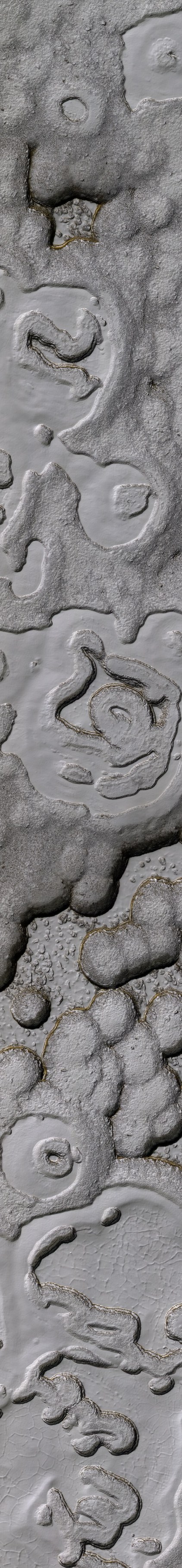
Finally: the picture at the start of This Week's Finds shows dry ice - frozen carbon dioxide - on the south pole of Mars:

9) HiRISE (High Resolution Imaging Science Experiments), South polar residual cap monitoring: rare stratigraphic contacts, http://hirise.lpl.arizona.edu/ESP_014379_0925

This dry ice forms quite a variety of baroque patterns. I don't know how it happens! Here are couple more good pictures:

10) HiRISE (High Resolution Imaging Science Experiments), Evolution of the south polar residual cap, http://hirise.lpl.arizona.edu/PSP_004687_0930

11) HiRISE (High Resolution Imaging Science Experiments), South polar carbon dioxide ice cap, http://hirise.lpl.arizona.edu/ESP_014261_0930

Patrick Russell wrote a description of the last one:

This HiRISE image is of a portion of Mars' south polar residual ice cap. Like Earth, Mars has concentrations of water ice at both poles.

Because Mars is so much colder, however, the seasonal ice that gets deposited at high latitudes in the winter and is removed in the spring (generally analogous to winter-time snow on Earth) is actually carbon dioxide ice. Around the south pole there are areas of this carbon dioxide ice that do not disappear every spring, but rather survive winter after winter. This persistent carbon dioxide ice is called the south polar residual cap, and is what we are looking at in this HiRISE image.

Relatively high-standing smooth material is broken up by semi-circular depressions and linear, branching troughs that make a pattern resembling those of your fingerprints. The high-standing areas are thicknesses of several meters of carbon dioxide ice. The depressions and troughs are thought to be caused by the removal of carbon dioxide ice by sublimation (the change of a material from solid directly to gas). HiRISE is observing this carbon dioxide terrain to try to determine how these patterns develop and how fast the depressions and troughs grow.

While the south polar residual cap as a whole is present every year, there are certainly changes taking place within it. With the high resolution of HiRISE, we intend to measure the amount of expansion of the depressions over multiple Mars years. Knowing the amount of carbon dioxide removed can give us an idea of the atmospheric, weather, and climate conditions over the course of a year.

In addition, looking for where carbon dioxide ice might be being deposited on top of this terrain may help us understand if there is any net loss or accumulation of the carbon-dioxide ice over time, which would be a good indicator of whether Mars' climate is in the process of changing or not.

It looks like a white Christmas, just like the one they're having on the east coast of the United States! My mom lives in DC, and I need to call her and find out how she's doing, with all this snow.

Addenda: I wrote:

So, let's focus our attention on functions on |Sing(X)| that when restricted to any simplex give polynomials with rational coefficients. This is a commutative algebra over the rational numbers. Call it A.

Is it obvious that there are any such functions?

And indeed, we'd like this to work for any simplicial set. Given a simplicial set S, we can define an algebra A of real-valued functions on |S| that are rational polynomials when restricted to each simplex. Do the functions in A separate points of |S|?

Over at the n-Category Café we showed the answer is yes. The key lemma is this:

Conjecture: Suppose we are given an n-simplex and a continuous function f on its boundary which is a rational polynomial on each face. Then f extends to a rational polynomial on the whole n-simplex.

Maarten Bergvelt also caught a big mistake. I had thought the smooth 1-forms on smooth manifold were the same as the Kähler differentials for its algebra of smooth functions. Maarten doubted this - and David Speyer was able to prove it's wrong! (His proof uses the axiom of choice, since it involves a nonprincipal ultrafilter. Do we need the axiom of choice here?)

This led to a big discussion, which I've attempted to summarize in the above improved version of "week287". To see the discussion we had, and add your comments, visit n-Category Café.

We live on an island surrounded by a sea of ignorance. As our island of knowledge grows, so does the shore of our ignorance. - John Wheeler

© 2009 John Baez
baez@math.removethis.ucr.andthis.edu