


|
|
|
|
The last glacial period seemed to be ending quite nicely, things had warmed up a lot — but then, suddenly, the temperature in Europe dropped about 7 °C! In Greenland, it dropped about twice that much. In England it got so cold that glaciers started forming! In the Netherlands, in winter, temperatures regularly fell below -20 °C. Throughout much of Europe trees retreated, replaced by alpine landscapes, and tundra. The climate was affected as far as Syria, where drought punished the ancient settlement of Abu Hurerya. But it doesn't seem to have been a world-wide event.
This cold spell lasted for about 1300 years. And then, just as suddenly as it began, it ended! Around 9,500 BC, the temperature in Europe bounced back.
This episode is called the Younger Dryas, after a certain wildflower that enjoys cold weather, whose pollen is common in this period.
What caused the Younger Dryas? Could it happen again? An event like this could wreak havoc, so it's important to know. Alas, as so often in science, the answer to these questions is "we're not sure, but...."
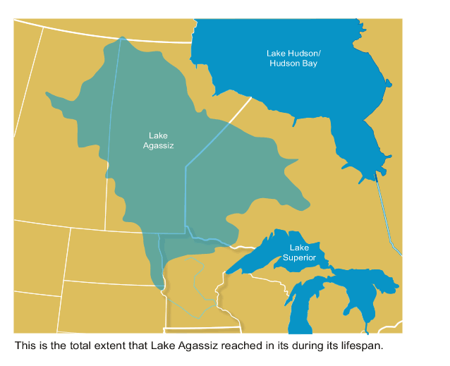
We're not sure, but the most popular theory is that a huge lake in Canada, formed by melting glaciers, broke its icy banks and flooded out into the Saint Lawrence River. This lake is called Lake Agassiz. At its maximum, it held more water than all lakes in the world now put together:
In a massive torrent lasting for years, the water from this lake rushed out to the Labrador Sea. By floating atop the denser salt water, this fresh water blocked a major current that flows in the Altantic: the Atlantic Meridional Overturning Circulation, or AMOC. This current brings warm water north and helps keep northern Europe warm. So, northern Europe was plunged into a deep freeze!
That's the theory, anyway.
Could something like this happen again? There are no glacial lakes waiting to burst their banks, but the concentration of fresh water in the northern Atlantic has been increasing, and ocean temperatures are changing too, so some scientists are concerned. The problem is, we don't really know what it takes to shut down the Atlantic Meridional Overturning Circulation!
To make progress on this kind of question, we need a lot of insight, but we also need some mathematical models. And that's what Nathan Urban will tell us about now. First we'll talk in general about climate models, Bayesian reasoning, and Monte Carlo methods. We'll even talk about the general problem of using simple models to study complex phenomena. And then he'll walk us step by step through the particular model that he and a coauthor have used to study this question: will the AMOC run amok?
Sorry, I couldn't resist that. It's not so much "running amok" that the AMOC might do, it's more like "fizzling out". But accuracy should never stand in the way of a good pun.
On with the show:
JB: Welcome back! Last time we were talking about the new work you're starting at Princeton. You said you're interested in the assessment of climate policy in the presence of uncertainties and "learning" - where new facts come along that revise our understanding of what's going on. Could you say a bit about your methodology? Or, if you're not far enough along on this work, maybe you could talk about the methodology of some other paper in this line of research.
NU: To continue the direction of discussion, I'll respond by talking about the methodology of a few papers along the lines of what I hope to work on here at Princeton, rather than about my past papers on uncertainty quantification. They are Keller and McInerney on learning rates:
• Klaus Keller and David McInerney, The dynamics of learning about a climate threshold, Climate Dynamics 30 (2008), 321-332.
Keller and coauthors on learning and economic policy:
• Klaus Keller, Benjamin M. Bolkerb and David F. Bradford, Uncertain climate thresholds and optimal economic growth, Journal of Environmental Economics and Management 48 (2004), 723-741.
and Oppenheimer et al. on "negative" learning (what happens when science converges to the wrong answer):
• Michael Oppenheimer, Brian C. O'Neill and Mort Webster, Negative learning, Climatic Change 89 (2008), 155-172.
The general theme of this kind of work is to statistically compare a climate model to observed data in order to understand what model behavior is allowed by existing data constraints. Then, having quantified the range of possibilities, plug this uncertainty analysis into an economic-climate model (or "integrated assessment model"), and have it determine the economically "optimal" course of action.
So: start with a climate model. There is a hierarchy of such models, ranging from simple impulse-response or "box" models to complex atmosphere-ocean general circulation models. I often use the simple models, because they're computationally efficient and it is therefore feasible to explore their full range of uncertainties. I'm moving toward more complex models, which requires fancier statistics to extract information from a limited set of time-consuming simulations.
Given a model, then apply a Monte Carlo analysis of its parameter space. Climate models cannot simulate the entire Earth from first principles. They have to make approximations, and those approximations involve free parameters whose values must be fit to data (or calculated from specialized models). For example, a simple model cannot explicitly describe all the possible feedback interactions that are present in the climate system. It might lump them all together into a single, tunable "climate sensitivity" parameter. The Monte Carlo analysis runs the model many thousands of times at different parameter settings, and then compares the model output to past data in order to see which parameter settings are plausible and which are not. I use Bayesian statistical inference, in combination with Markov chain Monte Carlo, to quantify the degree of "plausibility" (i.e., probability) of each parameter setting.
With probability weights for the model's parameter settings, it is now possible to weight the probability of possible future outcomes predicted by the model. This describes, conditional on the model and data used, the uncertainty about the future climate.
JB: Okay. I think I roughly understand this. But you're using jargon that may cause some readers' eyes to glaze over. And that would be unfortunate, because this jargon is necessary to talk about some very cool ideas. So, I'd like to ask what some phrases mean, and beg you to explain them in ways that everyone can understand.
To help out — and maybe give our readers the pleasure of watching me flounder around — I'll provide my own quick attempts at explanation. Then you can say how close I came to understanding you.
First of all, what's an "impulse-response model"? When I think of "impulse response" I think of, say, tapping on a wineglass and listening to the ringing sound it makes, or delivering a pulse of voltage to an electrical circuit and watching what it does. And the mathematician in me knows that this kind of situation can be modelled using certain familiar kinds of math. But you might be applying that math to climate change: for example, how the atmosphere responds when you pump some carbon dioxide into it. Is that about right?
NU: Yes. (Physics readers will know "impulse response" as "Green's functions", by the way).
The idea is that you have a complicated computer model of a physical system whose dynamics you want to represent as a simple model, for computational convenience. In my case, I'm working with a computer model of the carbon cycle which takes CO2 emissions as input and predicts how much CO2 is left in the air after natural sources and sinks operate on what's there. It's possible to explicitly model most of the relevant physical and biogeochemical processes, but it takes a long time for such a computer simulation to run. Too long to explore how it behaves under many different conditions, which is what I want to do.
How do you build a simple model that acts like a more complicated one? One way is to study the complex model's "impulse response" — in this case, how it behaves in response to an instantaneous "pulse" of carbon to the atmosphere. In general, the CO2 in the atmosphere will suddenly jump up, and then gradually relax back toward its original concentration as natural sinks remove some of that carbon from the atmosphere. The curve showing how the concentration decreases over time is the "impulse response". You derive it by telling your complex computer simulation that a big pulse of carbon was added to the air, and recording what it predicts will happen to CO2 over time.
The trick in impulse response theory is to treat an arbitrary CO2 emissions trajectory as the sum of a bunch of impulses of different sizes, one right after another. So, if emissions are 1, 3, and 7 units of carbon in years 1, 2, and 3, then you can think of that as a 1-unit pulse of carbon in year one, plus a 3-unit pulse in year 2, plus a 7-unit pulse in year 3.
The crucial assumption you make at this point is that you can treat the response of the complex model to this series of impulses as the sum of the "impulse response" curve that you worked out for a single pulse. Therefore, just by running the model in response to a single unit pulse, you can work out what the model would predict for any emissions trajectory, by adding up its response to a bunch of individual pulses. The impulse response model makes its prediction by summing up lots of copies of the impulse repsonse curve, with different sizes and at different times. (Techincally, this is a convolution of the impulse response curve, or Green's function, with the emissions trajectory curve.)
JB: Okay. Next, what's a "box model"? I had to look that up, and after some floundering around I bumped into a Wikipedia article that mentioned "black box models" and "white box models".
A black box model is where you've got a system, and all you pay attention to is its input and output — in other words, what you do to it, and what it does to you, not what's going on "inside". A white box model, or "glass box model", lets you see what's going on inside but not directly tinker with it, except via your input.
Is this at all close? I don't feel very confident that I've understood what a "box model" is.
NU: No, box models are the sorts of things you find in "systems dynamics" theory, where you have "stocks" of a substance and "flows" of it in and out. In the carbon cycle, the "boxes" (or stocks) could be "carbon stored in wood", "carbon stored in soil", "carbon stored in the surface ocean", etc. The flows are the sources and sinks of carbon. In an ocean model, boxes could be "the heat stored in the North Atlantic", "the heat stored in the deep ocean", etc., and flows of heat between them.
Box models are a way of spatially averaging over a lot of processes that are too complicated or time-consuming to treat in detail. They're another way of producing simplified models from more complex ones, like impulse response theory, but without the linearity assumption. For example, one could replace a three dimensional circulation model of the ocean with a couple of "big boxes of water connected by pipes". Of course, you have to then verify that your simplified model is a "good enough" representation of whatever aspect of the more complex model that you're interested in.
JB: Okay, sure — I know a bit about these "box models", but not that name. In fact the engineers who use "bond graphs" to depict complex physical systems made of interacting parts like to emphasize the analogy between electrical circuits and hydraulic systems with water flowing through pipes. So I think box models fit into the bond graph formalism pretty nicely. I'll have to think about that more.
Anyway: next you mentioned taking a model and doing a "Monte Carlo analysis of its parameter space". This time you explained what you meant, but I'll still go over it.
Any model has a bunch of adjustable parameters in it, for example the "climate sensitivity", which in a simple model just means how much warmer it gets per doubling of atmospheric carbon dioxide. We can think of these adjustable parameters as knobs we're allowed to turn. The problem is that we don't know the best settings of these knobs! And even worse, there are lots of allowed settings.
In a Monte Carlo analysis we randomly turn these knobs to some setting, run our model, and see how well it does — presumably by comparing its results to the "right answer" in some situation where we already know the right answer. Then we keep repeating this process. We turn the knobs again and again, and accumulate information, and try to use this to guess what the right knob settings are.
More precisely: we try to guess the probability that the correct knob settings lie within any given range! We don't try to guess their one "true" setting, because we can't be sure what that is, and it would be silly to pretend otherwise. So instead, we work out probabilities.
Is this roughly right?
NU: Yes, that's right.
JB: Okay. That was the rough version of the story. But then you said something a lot more specific. You say you "use Bayesian statistical inference, in combination with Markov chain Monte Carlo, to quantify the degree of "plausibility" (or probability) of each parameter setting."
So, I've got a couple more questions. What's "Markov chain Monte Carlo"? I guess it's some specific way of turning those knobs over and over again.
NU: Yes. For physicists, it's a "random walk" way of turning the knobs: you start out at the current knob settings, and tweak each one just a little bit away from where they currently are. In the most common Markov chain Monte Carlo (MCMC) algorithm, if the new setting takes you to a more plausible setting of the knobs, you keep that setting. If the new setting produces an outcome that is less plausible, then you might keep the new setting (with a likelihood proportional to how much less plausible the new setting is), or you might stay at the existing setting and try again with a new tweaking. The MCMC algorithm is designed so that the sequence of knob settings produced will sample randomly from the probability distribution you're interested in.
JB: And what's "Bayesian statistical inference"? I'm sorry, I know this subject deserves a semester-long graduate course. But like a bad science journalist, I will ask you to distill it down to a few sentences! Sometime I'll do a whole series of This Week's Finds about statistical inference, but not now.
NU: I can distill it to one sentence: in this context, it's a branch of statistics which allows you to assign probabilities to different settings of model parameters, based on how well those settings cause the model to reproduce the observed data.
The more common "frequentist" approach to statistics doesn't allow you to assign probabilities to model parameters. It has a different take on probability. As a Bayesian, you assume the observed data is known and talk about probabilities of hypotheses (here, model parameters). As a frequentist, you assume the hypothesis is known (hypothetically), and talk about probabilities of data that could result from it. They differ fundamentally in what you treat as known (data, or hypothesis) and what probabilities are applied to (hypothesis, or data).
JB: Okay, and one final question: sometimes you say "plausibility" and sometimes you say "probability". Are you trying to distinguish these, or say they're the same?
NU: I am using "probability" as a technical term which quantifies how "plausible" a hypothesis is. Maybe I should just stick to "probability".
JB: Great. Thanks for suffering through that dissection of what you said.
I think I can summarize, in a sloppy way, as follows. You take a model with a bunch of adjustable knobs, and you use some data to guess the probability that the right settings of these knobs lie within any given range. Then, you can use this model to make predictions. But these predictions are only probabilistic.
Okay, then what?
NU: This is the basic uncertainty analysis. There are several things that one can do with it. One is to look at learning rates. You can generate "hypothetical data" that we might observe in the future, by taking a model prediction and adding some "observation noise" to it. (This presumes that the model is perfect, which is not the case, but it represents a lower bound on uncertainty.) Then feed the hypothetical data back into the uncertainty analysis to calculate how much our uncertainty in the future could be reduced as a result of "observing" this "new" data. See Keller and McInerney for an example.
Another thing to do is decision making under uncertainty. For this, you need an economic integrated assessment model (or some other kind of policy model). Such a model typically has a simple description of the world economy connected to a simple description of the global climate: the world population and the economy grow at a certain rate which is tied to the energy sector, policies to reduce fossil carbon emissions have economic costs, fossil carbon emissions influence the climate, and climate change has economic costs. Different models are more or less explicit about these components (is the economy treated as a global aggregate or broken up into regional economies, how realistic is the climate model, how detailed is the energy sector model, etc.)
If you feed some policy (a course of emissions reductions over time) into such a model, it will calculate the implied emissions pathway and emissions abatement costs, as well as the implied climate change and economic damages. The net costs or benefits of this policy can be compared with a "business as usual" scenario with no emissions reductions. The net benefit is converted from "dollars" to "utility" (accounting for things like the concept that a dollar is worth more to a poor person than a rich one), and some discounting factor is applied (to downweight the value of future utility relative to present). This gives "the (discounted) utility of the proposed policy".
So far this has not taken uncertainty into account. In reality, we're not sure what kind of climate change will result from a given emissions trajectory. (There is also economic uncertainty, such as how much it really costs to reduce emissions, but I'll concentrate on the climate uncertainty.) The uncertainty analysis I've described can give probability weights to different climate change scenarios. You can then take a weighted average over all these scenarios to compute the "expected" utility of a proposed policy.
Finally, you optimize over all possible abatement policies to find the one that has the maximum expected discounted utility. See Keller et al. for a simple conceptual example of this applied to a learning scenario, and this book for a deeper discussion:
• William Nordhaus, A Question of Balance, Yale U. Press, New Haven, 2008.
It is now possible to start elaborating on this theme. For instance, in the future learning problem, you can modify the "hypothetical data" to deviate from what your climate model predicts, in order to consider what would happen if the model is wrong and we observe something "unexpected". Then you can put that into an integrated assessment model to study how much being wrong would cost us, and how fast we need to learn that we're wrong in order to change course, policy-wise. See that paper by Oppenheimer et al. for an example.
JB: Thanks for that tour of ideas! It sounds fascinating, important, and complex.
Now I'd like to move on to talking about a specific paper of yours. It's this one:
• Nathan Urban and Klaus Keller, Probabilistic hindcasts and projections of the coupled climate, carbon cycle, and Atlantic meridional overturning circulation system: A Bayesian fusion of century-scale observations with a simple model, Tellus A 62 (2010), 737-750.
Before I ask you about the paper, let me start with something far more basic: what the heck is the "Atlantic meridional overturning circulation" or "AMOC"?
I know it has something to do with ocean currents, and how warm water moves north near the surface of the Atlantic and then gets cold, plunges down, and goes back south. Isn't this related to the "Gulf Stream", that warm current that supposedly keeps Europe warmer than it otherwise would be?
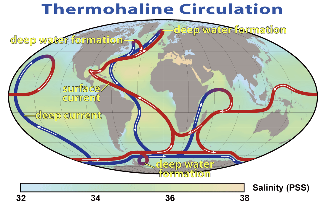
NU: Your first sentence pretty much sums up the basic dynamics: the warm water from the tropics cools in the North Atlantic, sinks (because it's colder and denser), and returns south as deep water. As the water cools, the heat it releases to the atmosphere warms the region.
This is the "overturning circulation". But it's not synonymous with the Gulf Stream. The Gulf Stream is a mostly wind-driven phenomenon, not a density driven current. The "AMOC" has both wind driven and density driven components; the latter is sometimes referred to as the "thermohaline circulation" (THC), since both heat and salinity are involved. I haven't gotten into salinity yet, but it also influences the density structure of the ocean, and you can read Stefan Rahmstorf's review articles for more (read the parts on non-linear behavior):
• Stefan Rahmstorf, The thermohaline ocean circulation: a brief fact sheet.
• Stefan Rahmstorf, Thermohaline ocean circulation, in Encyclopedia of Quaternary Sciences, edited by S. A. Elias, Elsevier, Amsterdam 2006.
JB: Next, why are people worrying about the AMOC? I know some scientists have argued that shortly after the last ice age, the AMOC stalled out due to lots of fresh water from Lake Agassiz, a huge lake that used to exist in what's now Canada, formed by melting glaciers. The idea, I think, was that this event temporarily killed the Gulf Stream and made temperatures in Europe drop enormously.
Do most people believe that story these days?
NU: You're speaking of the "Younger Dryas" abrupt cooling event around 11 to 13 thousand years ago. The theory is that a large pulse of fresh water from Lake Agassiz lessened the salinity in the Atlantic and made it harder for water to sink, thus shutting down down the overturning circulation and decreasing its release of heat in the North Atlantic. This is still a popular theory, but geologists have had trouble tracing the path of a sufficiently large supply of fresh water, at the right place, and the right time, to shut down the AMOC. There was a paper earlier this year claiming to have finally done this:
• Julian B. Murton, Mark D. Bateman, Scott R. Dallimore, James T. Teller and Zhirong Yang, Identification of Younger Dryas outburst flood path from Lake Agassiz to the Arctic Ocean, Nature 464 (2010), 740-743.
but I haven't read it yet.
The worry is that this could happen again — not because of a giant lake draining into the Atlantic, but because of warming (and the resulting changes in precipitation) altering the thermal and salinity structure of the ocean. It is believed that the resulting shutdown of the AMOC will cause the North Atlantic region to cool, but there is still debate over what it would take to cause it to shut down. It's also debated whether this is one of the climate "tipping points" that people talk about — whether a certain amount of warming would trigger a shutdown, and whether that shutdown would be "irreversible" (or difficult to reverse) or "abrupt".
Cooling Europe may not be a bad thing in a warming world. In fact, in a warming world, Europe might not actually cool in response to an AMOC shutdown; it might just warm more slowly. The problem is if the cooling is abrupt (and hard to adapt to), or prolonged (permamently shifting climate patterns relative to the rest of the world). Perhaps worse than the direct temperature change could be the impacts on agriculture or ocean ecosystems, resulting from major reorganizations of regional precipitation or ocean circulation patterns.
JB: So, part of your paper consists of modelling the AMOC and how it interacts with the climate and the carbon cycle. Let's go through this step by step.
First: how do you model the climate? You say you use "the DOECLIM physical climate component of the ACC2 model, which is an energy balance model of the atmosphere coupled to a one-dimensional diffusive ocean model". I guess these are well-known ideas in your world. But I don't even know what the acronyms stand for! Could you walk us through these ideas in a gentle way?
NU: Don't worry about the acronyms; they're just names people have given to particular models.
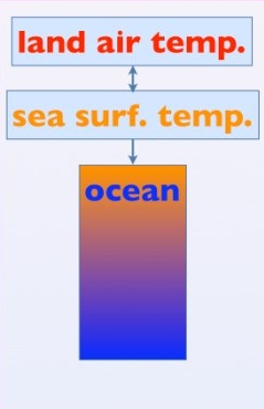
The ACC2 model is a computer model of both the climate and the carbon cycle. The climate part of our model is called DOECLIM, which I've used to replace the original climate component of ACC2. An "energy balance model" is the simplest possible climate model, and is a form of "box model" that I mentioned above. It treats the Earth as a big heat sink that you dump energy into (e.g., by adding greenhouse gases). Given the laws of thermodynamics, you can compute how much temperature change you get from a given amount of heat input.
This energy balance model of the atmosphere is "zero dimensional", which means that it treats the Earth as a featureless sphere, and doesn't attempt to keep track of how heat flows or temperature changes at different locations. There is no three dimensional circulation of the atmosphere or anything like that. The atmosphere is just a "lump of heat-absorbing material".
The atmospheric "box of heat" is connected to two other boxes, which are land and ocean. In DOECLIM, "land" is just another featureless lump of material, with a different heat capacity than air. The "ocean" is more complicated. Instead of a uniform box of water with a single temperature, the ocean is "one dimensional", meaning that it has depth, and temperature is allowed to vary with depth. Heat penetrates from the surface into the deep ocean by a diffusion process, which is intended to mimic the actual circulation-driven penetration of heat into the ocean. It's worth treating the ocean in more detail since oceans are the Earth's major heat sink, and therefore control how quickly the planet can change temperature.
The three parameters in the DOECLIM model which we treat as uncertain are the climate (temperature) sensitivity to CO2, the vertical mixing rate of heat into the ocean, and the strength of the "aerosol indirect effect" (what kind of cooling effect industrial aerosols in the atmosphere create due to their influence on cloud behavior).
JB: Okay, that's clear enough. But at this point I have to raise an issue about models in general. As you know, a lot of climate skeptics like to complain about the fallibility of models. They would surely become even more skeptical upon hearing that you're treating the Earth as a featureless sphere with same temperature throughout at any given time — and treating the temperature of ocean water as depending only on the depth, not the location. Why are you simplifying things so much? How could your results possibly be relevant to the real world?
Of course, as a mathematical physicist, I know the appeal of simple models. I also know the appeal of reducing the number of dimensions. I spent plenty of time studying quantum gravity in the wholly unrealistic case of a universe with one less dimension than our real world! Reducing the number of dimensions makes the math a lot simpler. And simplified models give us a lot of insight which — with luck — we can draw upon when tackling the really hard real-world problems. But we have to be careful: they can also lead us astray.
How do you think about results obtained from simplified climate models? Are they just mathematical warmup exercises? That would be fine — I have no problem with that, as long as we're clear about it. Or are you hoping that they give approximately correct answers?
NU: I use simple models because they're fast and it's easier to expose and explore their assumptions. My attitude toward simple models is a little of both the points of view you suggest: partly proof of concept, but also hopefully approximately correct, for the questions I'm asking. Let me first argue for the latter perspective.
If you're using a zero dimensional model, you can really only hope to answer "zero dimensional questions", i.e. about the globally averaged climate. Once you've simplified your question by averaging over a lot of the complexity of the data, you can hope that a simple model can reproduce the remaining dynamics. But you shouldn't just hope. When using simple models, it's important to test the predictions of their components against more complex models and against observed data.
You can show, for example, that as far as global average surface temperature is concerned, even simpler energy balance models than DOECLIM (e.g., without a 1D ocean) can do a decent job of reproducing the behavior of more complex models. See, e.g.:
• Isaac M. Held, Michael Winton, Ken Takahashi, Thomas Delworth, Fanrong Zeng and Geoffrey K. Vallis, Probing the fast and slow components of global warming by returning abruptly to preindustrial forcing, Journal of Climate 23 (2010), 2418-2427.
for a recent study. The differences between complex models can be captured merely by retuning the "effective parameters" of the simple model. For example, many of the complexities of different feedback effects can be captured by a tunable climate sensitivity parameter in the simple model, representing the total feedback. By turning this sensitivity "knob" in the simple model, you can get it to behave like complex models which have different feedbacks in them.
There is a long history in climate science of using simple models as "mechanistic emulators" of more complex models. The idea is to put just enough physics into the simple model to get it to reproduce some specific averaged behavior of the complex model, but no more. The classic "mechanistic emulator" used by the International Panel on Climate Change is called MAGICC. BERN-CC is another model frequently used by the IPCC for carbon cycle scenario analysis — that is, converting CO2 emissions scenarios to atmospheric CO2 concentrations. A simple model that people can play around with themselves on the Web may be found here:
• Ben Matthews, Chooseclimate.
Obviously a simple model cannot reproduce all the behavior of a more complex model. But if you can provide evidence that it reproduces the behavior you're interested in for a particular problem, it is arguably at least as "approximately correct" as the more complex model you validate it against, for that specific problem. (Whether the more complex model is an "approximately correct" representation of the real world is a separate question!)
In fact, simple models are arguably more useful than more complex ones for certain applications. The problem with complex models is, well, their complexity. They make a lot of assumptions, and it's hard to test all of them. Simpler models make fewer assumptions, so you can test more of them, and look at the sensitivity of your conclusions to your assumptions.
If I take all the complex models used by the IPCC, they will have a range of different climate sensitivities. But what if the actual climate sensitivity is above or below that range, because all the complex models have limitations? I can't easily explore that possibility in a complex model, because "climate sensitivity" isn't a knob I can turn. It's an emergent property of many different physical processes. If I want to change the model's climate sensitivity, I might have to rewrite the cloud physics module to obey different dynamical equations, or something complicated like that — and I still won't be able to produce a specific sensitivity. But in a simple model, "climate sensitivity" sensitivity is a "knob", and I can turn it to any desired value above, below, or within the IPCC range to see what happens.
After that defense of simple models, there are obviously large caveats. Even if you can show that a simple model can reproduce the behavior of a more complex one, you can only test it under a limited range of assumptions about model parameters, forcings, etc. It's possible to push a simple model too far, into a regime where it stops reproducing what a more complex model would do. Simple models can also neglect relevant feedbacks and other processes. For example, in the model I use, global warming can shut down the AMOC, but changes in the AMOC don't feed back to cool the global temperature. But the cooling from an AMOC weakening should itself slow further AMOC weakening due to global warming. The AMOC model we use is designed to partly compensate for the lack of explicit feedback of ocean heat transport on the temperature forcing, but it's still an approximation.
In our paper we discuss what we think are the most important caveats of our simple analysis. Ultimately we need to be able to do this sort of analysis with more complex models as well, to see how robust our conclusions are to model complexity and structural assumptions. I am working in that direction now, but the complexities involved might be the subject of another interview!
JB: I'd be very happy to do another interview with you. But you're probably eager to finish this one first. So we should march on.
But I can't resist one more comment. You say that models even simpler than DOECLIM can emulate the behavior of more complex models. And then you add, parenthetically, "whether the more complex model is an 'approximately correct' representation of the real world is a separate question!" But I think that latter question is the one that ordinary people find most urgent. They won't be reassured to know that simple models do a good job of mimicking more complicated models. They want to know how well these models mimic reality!
But maybe we'll get to that when we talk about the Monte Carlo Markov chain procedure and how you use that to estimate the probability that the "knobs" (that is, parameters) in your model are set correctly? Presumably in that process we learn a bit about how well the model matches real-world data?
If so, we can go on talking about the model now, and come back to this point in due time.
NU: The model's ability to represent the real world is the most important question. But it's not one I can hope to fully answer with a simple model. In general, you won't expect a model to exactly reproduce the data. Partly this is due to model imperfections, but partly it's due to random "natural variability" in the system. (And also, of course, to measurement error.) Natural variability is usually related to chaotic or otherwise unpredictable atmosphere-ocean interactions, e.g. at the scale of weather events, El Ni�o, etc. Even a perfect model can't be expected to predict those. With a simple model it's really hard to tell how much of the discrepancy between model and data is due to model structural flaws, and how much is attributable to expected "random fluctuations", because simple models are too simple to generate their own "natural variability".
To really judge how well models are doing, you have to use a complex model and see how much of the discrepancy can be accounted for by the natural variability it predicts. You also have to get into a lot of detail about the quality of the observations, which means looking at spatial patterns and not just global averages. This is the sort of thing done in model validation studies, "detection and attribution" studies, and observation system papers. But it's beyond the scope of our paper. That's why I said the best I can do is to use simple models that perform as well as complex models for limited problems. They will of course suffer any limitations of the complex models to which they're tuned, and if you want to read about those, you should read those modeling papers.
As far as what I can do with a simple model, yes, the Bayesian probability calculation using MCMC is a form of data-model comparison, in that it gives higher weight to model parameter settings that fit the data better. But it's not exactly a form of "model checking", because Bayesian probability weighting is a relative procedure. It will be quite happy to assign high probability to parameter settings that fit the data terribly, as long as they still fit better than all the other parameter settings. A Bayesian probability isn't an absolute measure of model quality, and so it can't be used to check models. This is where classical statistical measures of "goodness of fit" can be helpful. For a philosophical discussion, see:
• Andrew Gelman and Cosma Rohilla Shalizi, Philosophy and the practice of Bayesian statistics, available as arXiv:1006.3868.
That being said, you do learn about model fit during the MCMC procedure in its attempt to sample highly probable parameter settings. When you get to the best fitting parameters, you look at the difference between the model fit and the observations to get an idea of what the "residual error" is — that is, everything that your model wasn't able to predict.
I should add that complex models disagree more about the strength of the AMOC than they do about more commonly discussed climate variables, such as surface temperature. This can been seen in Figure 10.15 of the IPCC AR4 WG1 report: there is a cluster of models that all tend to agree with the observed AMOC strength, but there are also some models that don't. Some of those that don't are known to have relatively poor physical modeling of the overturning circulation, so this is to be expected (i.e., the figure looks like a worse indictment of the models than it really is). But there is still disagreement between some of the "higher quality" models. Part of the problem is that we have poor historical observations of the AMOC, so it's sometimes hard to tell what needs fixing in the models.
Since the complex models don't all agree about the current state of the AMOC, one can (and should) question using a simple AMOC model which has been tuned to a particular complex model. Other complex models will predict something altogether different. (And in fact, the model that our simple model was tuned to is also simpler than the IPCC AR4 models.) In our analysis we try to get around this model uncertainty by including some tunable parameters that control both the initial strength of the AMOC and how quickly it weakens. By altering those parameters, we try to span the range of possible outcomes predicted by complex models, allowing the parameters to take on whatever range of values is compatible with the (noisy) observations. This, at a minimum, leads to significant uncertainty in what the AMOC will do.
I'm okay with the idea of uncertainty — that is, after all, what my research is about. But ultimately, even projections with wide error bars still have to be taken with a grain of salt, if the most advanced models still don't entirely agree on simple questions like the current strength of the AMOC.
JB: Okay, thanks. Clearly the question of how well your model matches reality is vastly more complicated than what you started out trying to tell me: namely, what your model is. Let's get back to that.
To recap, your model consists of three interacting parts: a model of the climate, a model of the carbon cycle, and a model of the Atlantic meridional overturning circulation (or "AMOC"). The climate model, called "DOECLIM", itself consists of three interacting parts:
• the "land" (modeled as a "box of heat"),
• the "atmosphere" (modeled as a "box of heat")
• the "ocean" (modelled as a one-dimensional object, so that temperature varies with depth)
Next: how do you model the carbon cycle?
NU: We use a model called NICCS (nonlinear impulse-response model of the coupled carbon-cycle climate system). This model started out as an impulse response model, but because of nonlinearities in the carbon cycle, it was augmented by some box model components. NICCS takes fossil carbon emissions to the air as input, and calculates how that carbon ends up being partitioned between the atmosphere, land (vegetation and soil), and ocean.
For the ocean, it has an impulse response model of the vertical advective/diffusive transport of carbon in the ocean. This is supplemented by a differential equation that models nonlinear ocean carbonate buffering chemistry. It doesn't have any explicit treatment of ocean biology. For the terrestrial biosphere, it has a box model of the carbon cycle. There are four boxes, each containing some amount of carbon. They are "woody vegetation", "leafy vegetation", "detritus" (decomposing organic matter), and "humus" (more stable organic soil carbon). The box model has some equations describing how quickly carbon gets transported between these boxes (or back to the atmosphere).
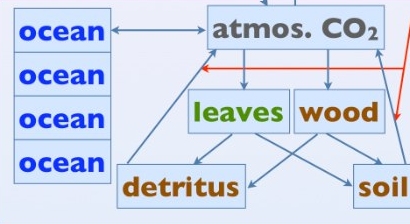
In addition to carbon emissions, both the land and ocean modules take global temperature as an input. (So, there should be a red arrow pointing to the "ocean" too — this is a mistake in the figure.) This is because there are temperature-dependent feedbacks in the carbon cycle. In the ocean, temperature determines how readily CO2 will dissolve in water. On land, temperature influences how quickly organic matter in soil decays ("heterotrophic respiration"). There are also purely carbon cycle feedbacks, such as the buffering chemistry mentioned above, and also "CO2 fertilization", which quantifies how plants can grow better under elevated levels of atmospheric CO2.
The NICCS model also originally contained an impulse response model of the climate (temperature as a function of CO2), but we removed that and replaced it with DOECLIM. The NICCS model itself is tuned to reproduce the behavior of a more complex Earth system model. The key three uncertain parameters treated in our analysis control the soil respiration temperature feedback, the CO2 fertilization feedback, and the vertical mixing rate of carbon into the ocean.
JB: Okay. Finally, how do you model the AMOC?
NU: This is another box model. There is a classic 1961 paper by Stommel:
• Henry Stommel, Thermohaline convection with two stable regimes of flow, Tellus 2 (1961), 224-230.
which models the overturning circulation using two boxes of water, one representing water at high latitudes and one at low latitudes. The boxes contain heat and salt. Together, temperature and salinity determine water density, and density differences drive the flow of water between boxes.
It has been shown that such box models can have interesting nonlinear dynamics, exhibiting both hysteresis and threshold behavior. Hysteresis means that if you warm the climate and then cool it back down to its original temperature, the AMOC doesn't return to its original state. Threshold behavior means that the system exhibits multiple stable states (such as an ocean circulation with or without overturning), and you can pass a "tipping point" beyond which the system flips from one stable equilibrium to another. Ultimately, this kind of dynamics means that it can be hard to return the AMOC to its historic state if it shuts down from anthropogenic climate change.
The extent to which the real AMOC exhibits hysteresis and threshold behavior remains an open question. The model we use in our paper is a box model that has this kind of nonlinearity in it:
• Kirsten Zickfeld, Thomas Slawig and Stefan Rahmstorf, A low-order model for the response of the Atlantic thermohaline circulation to climate change, Ocean Dynamics 54 (2004), 8-26.
Instead of Stommel's two boxes, this model uses four boxes:
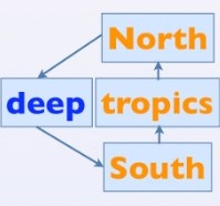
It has three surface water boxes (north, south, and tropics), and one box for an underlying pool of deep water. Each box has its own temperature and salinity, and flow is driven by density gradients between them. The boxes have their own "relaxation temperatures" which the box tries to restore itself to upon perturbation; these parameters are set in a way that attempts to compensate for a lack of explicit feedback on global temperature. The model's parameters are tuned to match the output of an intermediate complexity climate model.
The input to the model is a change in global temperature (temperature anomaly). This is rescaled to produce different temperature anomalies over each of the three surface boxes (accounting for the fact that different latitudes are expected to warm at different rates). There are similar scalings to determine how much freshwater input, from both precipitation changes and meltwater, is expected in each of the surface boxes due to a temperature change.
The main uncertain parameter is the "hydrological sensitivity" of the North Atlantic surface box, controlling how much freshwater goes into that region in a warming scenario. This is the main effect by which the AMOC can weaken. Actually, anything that changes the density of water alters the AMOC, so the overturning can weaken due to salinity changes from freshwater input, or from direct temperature changes in the surface waters. However, the former is more uncertain than the latter, so we focus on freshwater in our uncertainty analysis.
JB: Great! I see you're emphasizing the uncertain parameters; we'll talk more later about how you estimate these parameters, though you've already sort of sketched the idea.
So: you've described to me the three components of your model: the climate, the carbon cycle and the Atlantic meridional overturning current (AMOC). I guess to complete the description of your model, you should say how these components interact — right?
NU: Right. There is a two-way coupling between the climate module (DOECLIM) and the carbon cycle module (NICCS). The global temperature from the climate module is fed into the carbon cycle module to predict temperature-dependent feedbacks. The atmospheric CO2 predicted by the carbon cycle module is fed into the climate module to predict temperature from its greenhouse effect. There is a one-way coupling between the climate module and the AMOC module. Global temperature alters the overturning circulation, but changes in the AMOC do not themselves alter global temperature:
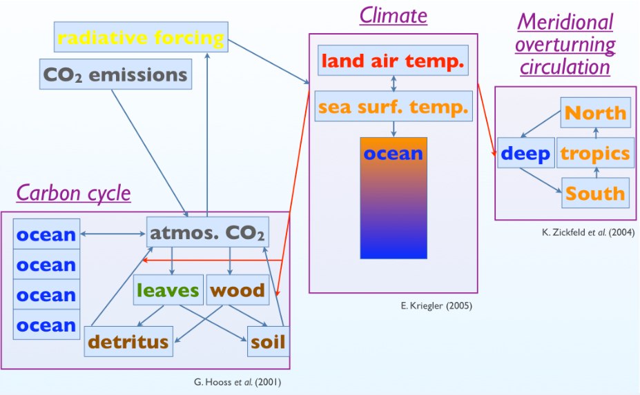
There is no coupling between the AMOC module and the carbon cycle module, although there technically should be: both the overturning circulation and the uptake of carbon by the oceans depend on ocean vertical mixing processes. Similarly, the climate and carbon cycle modules have their own independent parameters controlling the vertical mixing of heat and carbon, respectively, in the ocean. In reality these mixing rates are related to each other. In this sense, the modules are not fully coupled, insofar as they have independent representations of physical processes that are not really independent of each other. This is discussed in our caveats.
JB: There's one other thing that's puzzling me. The climate model treats the "ocean" as a single entity whose temperature varies with depth but not location. The AMOC model involves four "boxes" of water: north, south, tropical, and deep ocean water, each with its own temperature. That seems a bit schizophrenic, if you know what I mean. How are these temperatures related in your model?
You say "there is a one-way coupling between the climate module and the AMOC module." Does the ocean temperature in the climate model affect the temperatures of the four boxes of water in the AMOC model? And if so, how?
NU: The surface temperature in the climate model affects the temperatures of the individual surface boxes in the AMOC model. The climate model works only with globally averaged temperature. To convert a (change in) global temperature to (changes in) the temperatures of the surface boxes of the AMOC model, there is a "pattern scaling" coefficient which converts global temperature (anomaly) to temperature (anomaly) in a particular box.
That is, if the climate model predicts a 1 degree warming globally, that might be more or less than 1 °C of warming in the north Atlantic, tropics, etc. For example, we generally expect to see "polar amplification" where the high northern latitudes warm more quickly than the global average. These latitudinal scaling coefficients are derived from the output of a more complex climate model under a particular warming scenario, and are assumed to be constant (independent of warming scenario).
The temperature from the climate model which is fed into the AMOC model is the global (land+ocean) average surface temperature, not the DOECLIM sea surface temperature alone. This is because the pattern scaling coefficients in the AMOC model were derived relative to global temperature, not sea surface temperature.
JB: Okay. That's a bit complicated, but I guess some sort consistency is built in, which prevents the climate model and the AMOC model from disagreeing about the ocean temperature. That's what I was worrying about.
Thanks for leading us through this model. I think this level of detail is just enough to get a sense for how it works. And that I know roughly what your model is, I'm eager to see how you used it and what results you got!
But I'm afraid many of our readers may be nearing the saturation point. After all, I've been talking with you for days, with plenty of time to mull it over, while they will probably read this interview in one solid blast! So, I think we should quit here and continue in the next episode.
So, everyone: I'm afraid you'll just have to wait, clutching your chair in suspense, for the answer to the big question: will the AMOC get turned off, or not? Or really: how likely is such an event, according to this simple model?
For more discussion go to my blog, Azimuth.
...we're entering dangerous territory and provoking an ornery beast. Our climate system has proven that it can do very strange things. - Wallace S. Broecker
© 2010 John Baez
baez@math.removethis.ucr.andthis.edu
|
|
|
|