


|
|
|
|
I've been telling a long tale about analogies between different physical systems. Now I finally want to tell you about "bond graphs" - a technique engineers use to exploit these analogies. I'll just say a bit, but hopefully enough so you get the basic idea.
Then I'll sketch a rough classification of physical systems, and discuss the different kinds of math used to study these different kinds of systems. I'll only talk about systems from the realm of classical mechanics! To people who love classical field theory, quantum mechanics and quantum field theory, this may seem odd. Isn't classical mechanics completely understood?
Well, nothing is ever completely understood. But there are some reasons that mathematical physicists like myself tend to slip into thinking classical mechanics is better understood than it actually is. We love conservation of energy! Taking this seriously led to a wonderful framework called Hamiltonian mechanics, which we have been studying for over a century. We know a lot about that. We all studied it in school.
But the Hamiltonian mechanics we learn in school needs to be generalized a bit to nicely handle "dissipative systems", with friction - or more general "open systems", where energy can flow in and out of the boundary between the system and its environment.
(A dissipative system is really a special sort of open system, since energy lost to friction is really energy that goes into the environment. But the study of dissipative systems has not been fully integrated into the study of open systems! So, people often treat them separately, and I may do that too, now and then - even though it's probably dumb.)
Anyway, while lovers of beauty have the freedom to neglect dissipative systems and open systems if they want, engineers don't! Every machine interacts with its environment, and loses energy to its environment thanks to friction. Furthermore, machines are made of pieces, or "components". Each piece is an open system! Each component needs to be understood on its own... but then engineers need to understand how the components fit together and interact.
A lot of engineers do this with the help of "bond graphs". These are diagrams that describe systems made of various kinds of components: electrical, mechanical, hydraulic, chemical, and so on. The one thing all these components have in common is power. Energy can flow from one component to another. The rate of energy flow is called "power", and bond graphs are designed to make this easy to keep track of.
The idea behind bond graphs is very simple. I've been describing various "n-ports" lately, and I've drawn pictures of them. In my pictures, a 3-port looked like this:
      |  |  |
      V  V  V
      |  |  |
    -----------
   |           |
   |           |
    -----------
      |  |  |
      V  V  V
      |  |  |
In the case of an electrical system, this means 3 wires coming in and
3 going out. More generally, an n-port is a gadget with n inputs and
n outputs, where the flow into each input equals the flow out of the
corresponding output.
The idea of bond graphs is to draw these pictures differently. Don't draw individual wires! Instead, draw each pair of wires - input and output - as a single edge!
Such an edge is called a "bond". So, an n-port has n "bonds" coming out of it.
Take an electrical resistor, for example. This is a kind of 1-port - an example of what bond graph experts call a "resistance". Mathematically, a resistance is specified by a function relating effort to flow. In the example of an electrical resistor, effort is "voltage" and "flow" is current.
It's pretty natural to draw a resistor like this:
        |
        V
        |
      -----
     |     |
     |     |
      -----
        |
        V
        |
But in the world of bond graphs, people draw it more like this:
        |
        V
        |
      -----
     |     |
     |     |
      -----
One "bond" for two "wires"!
Actually, to be a bit more honest, they draw it a bit more like this:
           p'        \
    ------------------ R
           q'
Now the arrow is pointing across instead of down. There's a bond
coming in at the left, but nothing coming out at right. The p' and
q' let us know that the resistance is relating effort to flow. The
R stands for resistance.
To be even more honest, I should admit that most bond graph people use "e" for effort and "f" for flow. So, they really draw something like this:
           e        \
    ----------------- R
           f
But I want to stick with p' and q'.
Another famous 1-port is a capacitor. Bond graph people draw it like this:
           e        \
    ----------------- C
           f
A nice example of a 2-port is a transformer. I explained this
back in "week292".
Bond graph people draw it like this:
           e1     \           e2    \
    --------------- TF --------------
           f1                f2
There's a bond coming in at left and a bond coming out at right: 2
bonds for a 2-port. Similarly, a 3-port has 3 bonds coming out of it,
and so on. You'll see some 3-ports soon!
Bond graphs were invented by Henry Paynter. You can read his story here:
1) Henry M. Paynter, The gestation and birth of bond graphs, http://www.me.utexas.edu/~longoria/paynter/hmp/Bondgraphs.html
It reminds me slightly of Hamilton's story about inventing quaternions while walking down the river with his wife to a meeting of the Royal Irish Academy. Just slightly... but you can tell that bond graphs thrilled Paynter as much as quaternions thrilled Hamilton. I want to quote a bit, and comment on it. He begins:
Bond graphs were born in their present form on April 24, 1959. They were the direct outgrowth of my academic and professional experience during two previous decades. My MIT undergraduate and graduate training was centered on hydroelectric engineering, as was my work at Puget Power and my 8 years teaching in the Civil Engineering Department at MIT. This involved all aspects of the typical power plant indicated below.
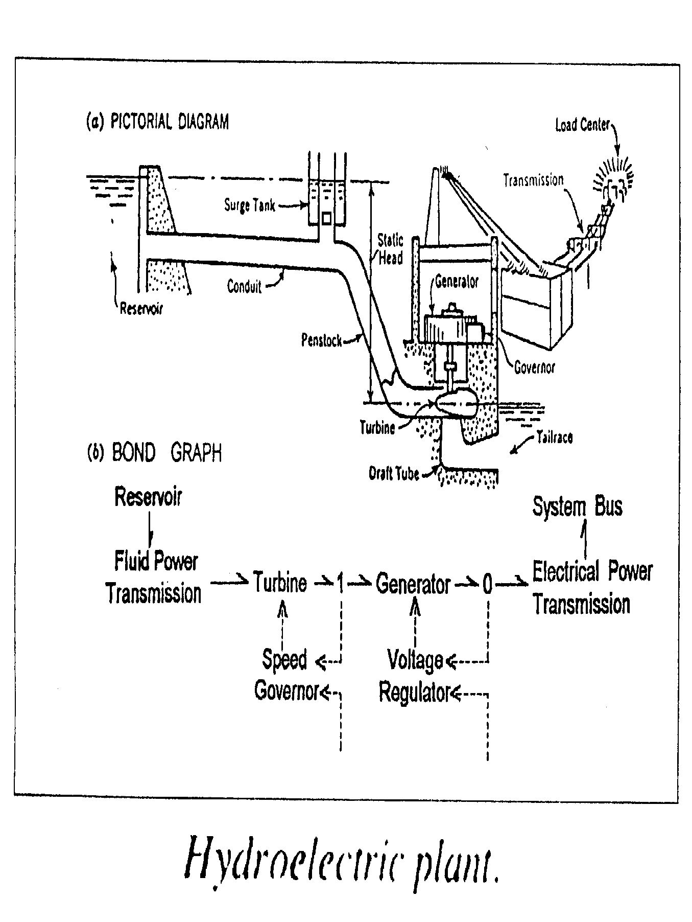
Here he shows a picture of a hydroelectric power plant, and the bond graph that abstractly describes it. A reservoir full of water acts as an "effort source", since water pressure is a form of "effort". Water flows down a conduit and turns a turbine. Here hydraulic power gets converted to mechanical power. Then the turbine turns a generator, which produces electricity - so here, mechanical power is getting converted to electrical power.
There are also some feedback loops, shown with dotted arrows. Solid arrows represent power, while dotted arrows represent "signals". For example, the turbine sends a signal about how fast it's turning to a a gadget called a "speed governor". If the turbine starts turning too fast or too slow, this gadget reduces or increases the flow of water to the turbine. There's a similar feedback loop involving the generator.
I haven't said anything about "signals" yet. The idea here is that information can be transmitted using negligible power. For example, you don't slow a turbine down much by attaching a little gadget that measures how fast it's turning. So, we can often get away with pretending that a signal carries no power. But this idealization breaks down in quantum mechanics - so if we ever get to talking about "quantum bond graphs", we'll have to rethink things. In fact, the idealization often breaks down long before quantum effects kick in! I think this aspect of bond graphs deserves more mathematical study.
You can see in Paynter's picture that the reservoir is a 1-port. It's an example of an "effort source" - a kind of 1-port I explained back in "week290". The turbine and generator are 2-ports, since they have an input and output. These are both "transformers" - a kind of 2-port I explained last week. You'll also see that the feedback loops involve some 3-ports. I explained these too last week. The 0 stands for a "parallel junction", and the 1 stands for a "series junction".
Paynter continues:
This training and experience in hydroelectric power actually forced certain insights upon me, most particularly an awareness of the strong analogies existing between:But Paynter only got the idea of bond graphs when he moved from the civil engineering department to the mechanical engineering department at MIT. Then comes the part that reminds me of Hamilton's famous description of inventing the quaternions. In a letter to his pal Tait, Hamilton wrote:TRANSMISSION (fluid pipes & electric lines);
TRANSDUCTION (turbines & generators);
CONTROL (speed governors & voltage regulators).When these analogous devices were reduced to equations for computer simulation, distinctions became completely blurred.
Even before 1957 it was obvious that the above hydroelectric plant necessarily involved two energy-converting transduction multiports: the hydraulic turbine converting fluid power to rotary shaft power and the electrical generator converting this shaft power into polyphase AC power. Moreover, the strict analogy between these two devices holds right down to the local field-continuum level. Thus the fluid vorticity corresponds precisely to the current density and the fluid circulation to the magnetizing current, so that even the turbine blades correspond to the generator pole pieces! In dynamic consequence, both these highly efficient components become 2-port gyrators, with parasitic losses. Common sense dictated that such compelling analogies implied some underlying common generalization from which other beneficial specializations might ensue. My efforts were also strongly motivated by a preoccupation with the logical philosophy underlying analogies in general. Such concerns were much earlier formalized by the mathematician, Eliakim Hastings Moore, in the following dictum:
"We lay down a fundamental principle of generalization by abstraction: The existence of analogies between central features of various theories implies the existence of a general theory which underlies the particular theories and unifies them with respect to those central features... "
To-morrow will be the 15th birthday of the Quaternions. They started into life, or light, full grown, on the 16th of October, 1843, as I was walking with Lady Hamilton to Dublin, and came up to Brougham Bridge, which my boys have since called the Quaternion Bridge. That is to say, I then and there felt the galvanic circuit of thought close; and the sparks which fell from it were the fundamental equations between i, j, k; exactly such as I have used them ever since. I pulled out on the spot a pocket-book, which still exists, and made an entry, on which, at the very moment, I felt that it might be worth my while to expend the labour of at least ten (or it might be fifteen) years to come. But then it is fair to say that this was because I felt a problem to have been at that moment solved - an intellectual want relieved - which had haunted me for at least fifteen years before.
Paynter writes:
In 1954, I moved over to the MIT mechanical engineering department to establish the first systems engineering subjects at MIT. It was this specific task which 5 years later produced bond graphs, drawing naturally upon all the attitudes and experience indicated above. So it was on April 24, 1959, when I was to deliver the lecture as posted below, I awoke that morning with the idea of the 0,1-junctions somehow planted in my head overnight! Moreover the very symbols (0,1) for Kirchoff's current law and Kirchoff's voltage law, respectively, made direct the correspondence between circuit duality and logical duality. (The limited use of these 3-ports in the hydro plant bond graph above hardly does justice to their role in rendering bond graphs a complete and formal discipline.)

(If you don't understand what Paynter means by Kirchoff's current law and Kirchoff's voltage law, and "the correspondence between circuit duality and logical duality", you can see a bit of explanation in the Addenda.)
Paynter's book on bond graphs came out in 1961:
2) Henry M. Paynter, Analysis and Design of Engineering Systems, MIT Press, Cambridge, Massachusetts, 1961.
About a decade later, bond graphs were taken up by many others authors, notably Jean Thoma:
3) Jean U. Thoma, Introduction to Bond Graphs and Their Applications, Pergamon Press, Oxford, 1975.
By now there is a vast literature on bond graphs. This website is a bit broken, but you can use it to get a huge bibliography:
4) Bondgraph.info, Journal articles, http://www.bondgraph.info/journal.html
Books, http://www.bondgraph.info/books.html
I've listed some of my favorite books in previous Weeks. But if you want an online introduction to bond graphs, start here:
5) Wikipedia, Bond graph, http://en.wikipedia.org/wiki/Bond_graph
It covers a topic I haven't even mentioned, the "causal stroke". And it gives some examples of how to convert bond graphs into differential equations. If you read the talk page for this article, you'll see that various people have found it confusing at various times. But it's gotten a lot clearer since then, and I hope people keep improving it. I'll probably work on it myself a bit.
Then, watch some of these:
6) Soumitro Banerjee, Dynamics of physical systems, lectures on YouTube. Lectures 13-19: The bond graph approach. Available at http://www.youtube.com/view_play_list?p=D074EEC1EBEFAEA5
These lectures are very thoughtful and nice. I thank C. J. Fearnley for pointing them out.
Now I'd like to veer off in a slightly different direction, and ponder the various n-ports we've seen, and how they fit into different branches of mathematical physics. My goal is to dig a bit deeper into the mathematics behind this big analogy chart:
                displacement    flow          momentum      effort
                     q           q'              p            p'

Mechanics       position       velocity       momentum      force
(translation)

Mechanics       angle          angular        angular       torque
(rotation)                     velocity       momentum

Electronics     charge         current        flux          voltage
                                              linkage

Hydraulics      volume         flow           pressure      pressure
                                              momentum

Thermodynamics  entropy        entropy        temperature   temperature
                               flow           momentum

Chemistry       moles          molar          chemical      chemical
                               flow           momentum      potential
But I won't be using the language of bond graphs! The reason is that I want to talk about gizmos where the total number of inputs and outputs can be either even or odd, like this:
        |
        |
      -----
     |     |
      -----
      /   \
     /     \
Even though I'm talking about all sorts of physical systems, I'll use
the language of electronics, and call these gizmos "circuit
elements". We can stick these together to form
"circuits", like this:
        |           |
        |           |
      -----         |
     |     |        |
      -----         |
      /   \         |
     /     \        |
  ------------      |
 |            |     |
  ------------      |
    |  |  |         |
    |  |   \_______/
    |  |
    |  |
Category theorists will instantly see that circuits are morphisms in
something like a compact closed symmetric monoidal category! But the
rest of you shouldn't worry your pretty heads about that yet. The main
thing to note is that we have "open" circuits that have wires coming
in and out, as above, but also "closed" ones that don't, like this:
          _________
         /         \
        |           |
        |           |
      -----         |
     |     |        |
      -----         |
      /   \         |
     /     \        |
  ------------      |
 |            |     |
  ------------      |
    |  |  |         |
    |  |   \_______/
    |  |
   ------
  |      |
   ------
I will also call circuits "systems", since that's what
physicists call them. And indeed, they often speak of
"closed" systems, which don't interact with their
environment, or "open" ones, which do.
We've seen different kinds of circuit elements. First there are "active" circuit elements, which can absorb and emit energy, and for which we cannot define a Hamiltonian that makes energy conserved. Then there are "passive" ones, which come in two kinds:
Not surprisingly, circuits made of different kinds of circuit elements want to be studied in different ways! We get pulled into all sorts of nice mathematics this way - especially symplectic geometry, Hodge theory, and complex analysis. Here's a quick survey:
By using a Legendre transform, we can compute p as a function of q'. Then we can work out the "Hamiltonian" of our circuit, as follows:
H(p,q) = L(q,q') - p.q'
Like the Lagrangian, this Hamiltonian will be the sum of Hamiltonians for each piece - and I've told you what those Hamiltonians are for all the conservative circuit elements I've mentioned.
If the overall circuit is closed, no wires coming in or going out, its Hamiltonian will be conserved in the strongest sense:
dH/dt = 0
There are elegant ways to study closed systems using Hamiltonian mechanics - or in other words, symplectic geometry. This is something mathematical physicists know well.
We can also examine the special case of a conservative closed system in a static state, meaning that p and q don't depend on time. The behavior of such systems is governed by the PRINCIPLE OF LEAST ENERGY: it will choose p and q that minimize the Hamiltonian H(q,p).
If the circuit is open, we need a slight generalization of Hamiltonian mechanics that can handle systems that interact with their environment. Open systems are less familiar in mathematical physics - but as I explained in "week290", they're studied in "control theory". Open systems obey a weaker form of energy conservation, called the "power balance equation".
p'.q'
Using this we can often solve for q' as a function of p' or vice versa.
The principal of least power is closely related to other minimum principles in physics. For example, if we build a network of resistors and fix the voltages on the wires coming in and out, the voltages on the network will obey a discretized version of the Laplace equation. This is the equation a function f satisfies when it minimizes
∫ (∇f)2
So, circuits of this second kind are closely related to the Laplace equation, differential forms, Hodge theory and the like. In fact this is why Raoul Bott switched from electrical engineering to differential topology!
q' = Ap'
Or, we can take the inverse of this operator and get the "impedance matrix", which tells us the flows as a function of the efforts:
p' = Zq'
Here both efforts and flows are functions of time. Taking a Fourier transform in the time variable we get a version of the impedance matrix that's a function of the dual variable: "frequency". And if the circuit is built from linear resistances and inertances, we'll get a rational function of frequency! The poles of this function contain juicy information. So, we can use complex analysis to study such circuits. This is very standard stuff in electrical engineering.
p' = Aq' + e
where e comes from the effort sources. This is called Norton's theorem. Alternatively we can write
q' = Zp' + f
where f comes from the flow sources. This is called Th�venin's theorem. Again, these are standard results that electrical engineers learn - but don't forget, they apply to all the systems in our chart of analogies!
I hope in future Weeks to say more about this stuff. I hope you see there are some strange and interesting patterns here - like this trio:
THE PRINCIPLE OF LEAST ACTION
THE PRINCIPLE OF LEAST ENERGY
THE PRINCIPLE OF LEAST POWER
We've seen the trio of action, energy and power before, back in "week289". Action has units of energy × time; power has units of energy/time. How do these three minimum principles fit together in a unified whole? I know how to derive the principal of least energy from the principle of least action by starting with a conservative system and imposing the assumption that it's static. But how about the principle of least power? Where does this come from?
I don't know. If you know, tell me!
I'll tell you a bit about linear dissipative circuits and Hodge theory next week. But if you're impatient to learn circuit theory - or at least know what books are lying next to my bed - let me give some references!
This book is quite good:
7) Brian D. O. Anderson and Sumeth Vongpanitlerd, Network Analysis and Synthesis: A Modern Systems Theory Approach, Dover Publications, Mineola, New York, 2006.
There's a lot of complex analysis in here! Some is familiar, but there's also a lot we mathematicians don't usually learn: the Positive Real Lemma, the Bounded Real Lemma, and more.
Speaking of Norton's and Th�venin's theorems, these articles demystify those:
8) Wikipedia, Norton's theorem, http://en.wikipedia.org/wiki/Norton%27s_theorem
9) Wikipedia, Th�venin's theorem, http://en.wikipedia.org/wiki/Th%C3%A9venin%27s_theorem
These articles cover only circuits with one input and one output which are made from flow sources, effort sources and linear resistances. I know the results generalize to circuits where we also allow capacticances and inertances, and above I was willing to wager that they apply to circuits with as many inputs and outputs as you like.
This book of classic papers is also good:
10) M. E. van Valkenburg, ed., Circuit Theory: Foundations and Classical Contributions, Dowden, Hutchington and Ross, Stroudsburg, Pennsylvania, 1974.
I mentioned Raoul Bott - mathematicians will be pleased and perhaps surprised to see a 1948 paper by him here! It's 5 paragraphs long, and it solved a basic problem.
Addenda: Joris Vankerschaver writes:
I've been following TWF the past few weeks extra carefully since I'm also interested in a systematic approach of electrical circuits, mechanical systems, and the like. For this issue of TWF, I was wondering if you know whether there is a link between the Hamilton-Pontryagin (HP) variational principle and the action principles you mentioned. I hope you don't mind me asking a direct question like this...Unfortunately I had to tell him that I've never heard of the Hamilton-Pontryagin variational principle. More to learn!The HP principle consists of taking a Lagrangian L(q, v), and thinking of v as an extra coordinate. We then add the condition that q' = v as an extra constraint with a Lagrange multiplier p, to get a functional of the form
S(q, v, p) = ∫ p (q' - v) + L(q, v) dt
where q, v, p are varied independently. The result is the Euler-Lagrange equations in implicit form, together with Hamilton's equations and the Legendre transformation.
I've added a PDF draft where these calculations are done in more detail.
H. Yoshimura (who is a classical bond grapher) and J. Marsden have been working on this variational principle and apparently used it to great effect in circuit theory as well. Circuits typically have degenerate Lagrangians and nonholonomic constraints, and the HP principle handles these very well. But the HP variational principle has been re-discovered many times before.
The equations of motion obtained from the HP principle can also be incorporated into a Dirac structure, which (according to van der Schaft and Maschke) is very well suited for interconnection purposes (where power is conserved). So again, I was wondering if there was a link between the HP principle and what you are considering.
I would be very interested in hearing your thoughts about this. I am really looking forward to the next few issues of TWF!
In "week292" I briefly mentioned the "dual" of a planar electrical circuit, where we switch series junctions and parallel junctions, switch efforts (voltages) and flows (currents), and so on. You'll note that in my quote of Paynter he was drawing a perhaps slightly obscure analogy between this sort of duality and what he called "logical" duality. This is usually called "De Morgan duality": it's a symmetry of classical logic, which consists of switching true and false, AND and OR, and so on. In binary notation it consists of switching 0 and 1. This is why Paynter called a parallel junction a "0-junction" and the series junction a "1-junction". I didn't really understand the connection until Chris Weed explained it:
John,Francesco La Tella writes:The point is pretty trivial, but it's perhaps worth reminding the reader of the immediate connection to the dualities of Boolean algebra.
More precisely, a series connection of two switches can be considered to implement the function AND(x,y) - defined by the usual truth table - if one encodes 'True' as a closed connection and 'False' as an open connection. Of course, this can be considered a convention. If 'True' is encoded by an open connection and 'False' is encoded by a closed connection, then a series connection of the switches implements OR(x,y).
Of course, the "dual" of this little exposition applies to a parallel connection.
I have a continuing interest in these simple observations in connection with an idea that I attempted to present in a post on Math Overflow. For understandable reasons, it didn't generate much of a response. Perhaps a few people were motivated to chew on it for a while.
— Chris
Greetings John,I am having fun reading about bond graphs (in an attempt to stay awake during the graveyard shift at work) on your site.
With regard to the principle of least power (PLP). I remember writing an assignment for the subject of Optimization II, in my senior year of an undergraduate maths degree. Basically we were asked to use mathematical optimization techniques to model an appropriate physical, industrial, financial, etc. system in order to determine optimal operational parameters or values. Most of my classmates chose typical, classic, textbook problems from one of the many fine textbooks available to us. However, having had a vague recollection, at the time, to a reference in a 1989 (circa?) issue of Electronics & Wireless World which touched on this very subject, I got to digging.
In brief, it turns out that, the distributions of voltages and currents in electrical networks (circuits), containing both active and passive circuit elements, can be solved for by using a stationary-power-condition dictated by the principle of least power. Using this idea an objective function is formulated in which each term describes the power dissipated in each of the circuit elements comprising the network. Since the objective is bivariate, one only needs to find the stationary point in this "power manifold" to determine the real, physical values of currents and voltages in and around all circuit elements.
The situation is only slightly complicated by the presence of active and reactive circuit elements, but is covered sufficiently by a generalized version of this concept.
Over the years I've had occasion to mention this alternative technique for circuit analysis to many of my electrical engineer colleagues and friends, only to be surprised that ALL were blissfully unaware of this very elegant yet very useful solution. It's unfortunate that engineers today are taught nodal analysis (Kirchhoff's current law & Kirchoff's voltage law), a little linear algebra and perhaps some physics, certainly lots of experience using circuit-CAD packages, but no time exploring alternative possibilities. In contrast ALL my physicist friends are intuitively, if not explicitly attuned to the existence of the unifying power of the three principles PLA, PLE and PLP, and all their possibilities.
Thank you for helping to keep my brain cells active.
Kind regards,
Francesco La Tella
For more discussion, visit the n-Category Café.
I was born not knowing and have had only a little time to change that here and there - Richard Feynman
© 2010 John Baez
baez@math.removethis.ucr.andthis.edu
|
|
|
|