


|
|
|
|
In the next issues of This Week's Finds, I'll return to interviewing people who are trying to help humanity deal with some of the risks we face.
First I'll talk to the science fiction author and astrophysicist Gregory Benford. I'll ask him about his ideas on "geoengineering" — proposed ways of deliberately manipulating the Earth's climate to counteract the effects of global warming.
After that, I'll spend a few weeks asking Eliezer Yudkowsky about his ideas on rationality and "friendly artificial intelligence". Yudkowsky believes that the possibility of dramatic increases in intelligence, perhaps leading to a technological singularity, should command more of our attention than it does.
Needless to say, all these ideas are controversial. They're exciting to some people — and infuriating, terrifying or laughable to others. But I want to study lots of scenarios and lots of options in a calm, level-headed way without rushing to judgement. I hope you enjoy it.
This week, I want to say a bit more about the Hopf bifurcation!
Last week I talked about applications of this mathematical concept to climate cycles like the El Niño - Southern Oscillation. But over on the Azimuth Project, Graham Jones has explained an application of the same math to a very different subject:
• Quantitative ecology, Azimuth Project.
That's one thing that's cool about math: the same patterns show up in different places. So, I'd like to take advantage of his hard work and show you how a Hopf bifurcation shows up in a simple model of predator-prey interactions.
Suppose we have some rabbits that reproduce endlessly, with their numbers growing at a rate proportional to their population. Let $x(t)$ be the number of animals at time $t$. Then we have:
\[ \frac{d x}{d t} = r x \]
where $r$ is the growth rate. This gives exponential growth: it has solutions like
\[ x(t) = x_0 e^{r t} \]
To get a slightly more realistic model, we can add 'limits to growth'. Instead of a constant growth rate, let's try a growth rate that decreases as the population increases. Let's say it decreases in a linear way, and drops to zero when the population hits some value $K$. Then we have
\[ \frac{d x}{d t} = r (1-x/K) x \]
This is called the "logistic equation". $K$ is known as the "carrying capacity". The idea is that the environment has enough resources to support this population. If the population is less, it'll grow; if it's more, it'll shrink.
If you know some calculus you can solve the logistic equation by hand by separating the variables and integrating both sides; it's a textbook exercise. The solutions are called "logistic functions", and they look sort of like this:

The above graph shows the simplest solution:
\[ x = \frac{e^t}{e^t + 1} \]
of the simplest logistic equation in the world:
\[ \frac{ d x}{d t} = (1 - x)x \]
Here the carrying capacity is 1. Populations less than 1 sound a bit silly, so think of it as 1 million rabbits. You can see how the solution starts out growing almost exponentially and then levels off. There's a very different-looking solution where the population starts off above the carrying capacity and decreases. There's also a silly solution involving negative populations. But whenever the population starts out positive, it approaches the carrying capacity.
The solution where the population just stays at the carrying capacity:
\[ x = 1 \]
is called a "stable equilibrium", because it's constant in time and nearby solutions approach it.
But now let's introduce another species: some wolves, which eat the rabbits! So, let $x$ be the number of wolves, and $y$ the number of rabbits. Before the rabbits meet the wolves, let's assume they obey the logistic equation:
\[ \frac{d x}{d t} = x(1-x/K) \]
And before the wolves meet the rabbits, let's assume they obey this equation:
\[ \frac{d y}{d t} = -y \]
so that their numbers would decay exponentially to zero if there were nothing to eat.
So far, not very interesting. But now let's include a term that describes how predators eat prey. Let's say that on top of the above effect, the predators grow in numbers, and the prey decrease, at a rate proportional to:
\[ x y/(1+x). \]
For small numbers of prey and predators, this means that predation increases nearly linearly with both $x$ and $y$. But if you have one wolf surrounded by a million rabbits in a small area, the rate at which it eats rabbits won't double if you double the number of rabbits! So, this formula includes a limit on predation as the number of prey increases.
Okay, so let's try these equations:
\[ \frac{ d x}{d t} = x(1-x/K) - 4x y/(x+1) \]
and
\[ \frac{ d y}{d t} = -y + 2x y/(x+1) \]
The constants 4 and 2 here have been chosen for simplicity rather than realism.
Before we plunge ahead and get a computer to solve these equations, let's see what we can do by hand. Setting $d x/d t = 0$ gives the interesting parabola
\[ y = \frac{1}{4}(1-x/K)(x+1) \]
together with the boring line $x = 0$. (If you start with no prey, that's how it will stay. It takes bunny to make bunny.)
Setting $d y/d t = 0$ gives the interesting line
\[ x=1 \]
together with the boring line $y = 0$.
The interesting parabola and the interesting line separate the $x y$ plane into four parts, so these curves are called separatrices. They meet at the point
\[ y = \frac{1}{2} (1 - 1/K) \]
which of course is an equilibrium, since $d x / d t = d y / d t = 0$ there. But when $K < 1$ this equilibrium occurs at a negative value of $y$, and negative populations make no sense.
So, if $K < 1$ there is no equilibrium population, and with a bit more work one can see the problem: the wolves die out. For larger values of $K$ there is an equilibrium population. But the nature of this equilibrium depends on $K$: that's the interesting part.
We could figure this out analytically, but let's look at two of Graham's plots. Here's a solution when $K = 2.5$:

The gray curves are the separatrices. The red curve shows a solution of the equations, with the numbers showing the passage of time. So, you can see that the solution spirals in towards the equilibrium. That's what you expect of a stable equilibrium.
Here's a picture when $K = 3.5$:

The red and blue curves are two solutions, again numbered to show how time passes. The red curve spirals in towards the dotted gray curve. The blue one spirals out towards it. The gray curve is also a solution. It's called a "stable limit cycle" because it's periodic, and nearby solutions move closer and closer to it.
With a bit more work, we could show analytically that whenever $1 < K < 3$ there is a stable equilibrium. As we increase $K$, when $K$ passes 3 this stable equilibrium suddenly becomes a tiny stable limit cycle. This is a Hopf bifurcation!
Now, what if we add noise? We saw the answer last week: where we before had a stable equilibrium, we now can get irregular cycles — because the noise keeps pushing the solution away from the equilibrium!
Here's how it looks for $K=2.5$ with white noise added:

The following graph shows a longer run in the noisy $K=2.5$ case, with rabbits ($x$) in black and wolves ($y$) in gray.

There is irregular periodicity — and as you'd expect, the predators tends to lag behind the prey. A burst in the rabbit population causes a rise in the wolf population; a lot of wolves eat a lot of rabbits; a crash in rabbits causes a crash in wolves.
This sort of phenomenon is actually seen in nature sometimes. The most famous case involves the snowshoe hare and the lynx in Canada. It was first noted by MacLulich:
The snowshoe hare is also known as the "varying hare", because its coat varies in color quite dramatically. In the summer it looks like this:

In the winter it looks like this:

The Canada lynx is an impressive creature:

But don't be too scared: it only weighs 8-11 kilograms, nothing like a tiger or lion.
Down in the United States, the same species lynx went extinct in Colorado around 1973 — but now it's back!
• Colorado Division of Wildlife, Success of the Lynx Reintroduction Program, 27 September, 2010.
In Canada, at least, the lynx rely for the snowshoe hare for 60% to 97% of their diet. I suppose this is one reason the hare has evolved such magnificent protective coloration. This is also why the hare and lynx populations are tightly coupled. They rise and crash in irregular cycles that look a bit like what we saw in our simplified model:
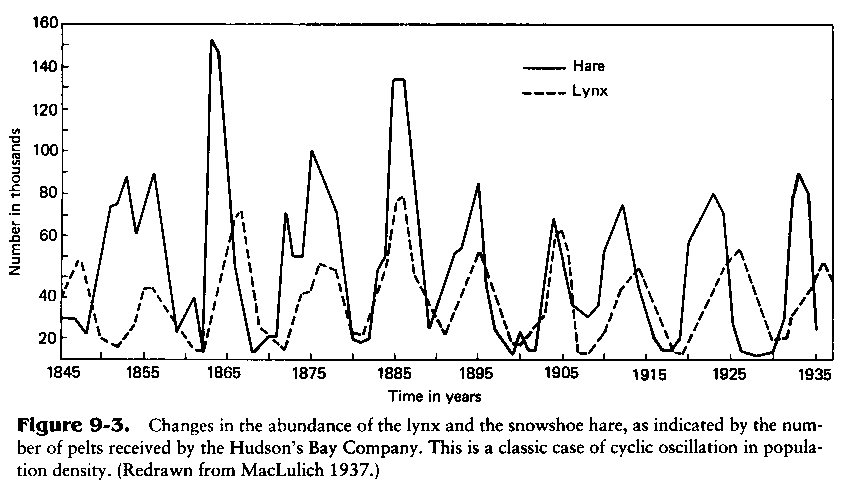
This cycle looks a bit more strongly periodic than Graham's graph, so to fit this data, we might want to choose parameters that give a limit cycle rather than a stable equilibrium.
But I should warn you, in case it's not obvious: everything about population biology is infinitely more complicated than the models I've showed you so far! Some obvious complications: snowshoe hare breed in the spring, their diet varies dramatically over the course of year, and the lynx also eat rodents and birds, carrion when it's available, and sometimes even deer. Some less obvious ones: the hare will eat dead mice and even dead hare when they're available, and the lynx can control the size of their litter depending on the abundance of food. And I'm sure all these facts are just the tip of the iceberg. So, it's best to think of models here as crude caricatures designed to illustrate a few features of a very complex system.
I hope someday to say a bit more and go a bit deeper. Do any of you know good books or papers to read, or fascinating tidbits of information? Graham Jones recommends this book for some mathematical aspects of ecology:
• Michael R. Rose, Quantitative Ecological Theory, Johns Hopkins University Press, Maryland, 1987.
Alas, I haven't read it yet.
Also: you can get Graham's R code for predator-prey simulations at the Azimuth Project.
For more discussion go to my blog, Azimuth.
Under carefully controlled experimental circumstances, the organism will behave as it damned well pleases. - the Harvard Law of Animal Behavior
© 2011 John Baez
baez@math.removethis.ucr.andthis.edu
|
|
|
|