


|
|
|
|
Last week we met the El Niño-Southern Oscillation, or ENSO. I like to explain things as I learn about them. So, often I look back and find my explanations naive. But this time it took less than a week!
What did it was reading this:
I wouldn't recommend this to the faint of heart. It's a bit terrifying. It's well-written, but it tells the long and tangled tale of how theories of the ENSO phenomenon evolved from 1969 to 1998 — a period that saw much progress, but did not end with a neat, clean understanding of this phenomenon. It's packed with hundreds of references, and sprinkled with somewhat intimidating remarks like:
The Fourier-decomposed longitude and time dependence of these eigensolutions obey dispersion relations familiar to every physical oceanographer...
Nonetheless I found it fascinating — so, I'll pick off one small idea and explain it now.
As I'm sure you've heard, climate science involves some extremely complicated models: some of the most complex known to science. But it also involves models of lesser complexity, like the "box model" explained by Nathan Urban in "week304". And it also involves some extremely simple models that are designed to isolate some interesting phenomena and display them in their Platonic ideal form, stripped of all distractions.
Because of their simplicity, these models are great for mathematicians to think about: we can even prove theorems about them! And simplicity goes along with generality, so the simplest models of all tend to be applicable — in a rough way — not just to the Earth's climate, but to a vast number of systems. They are, one might say, general possibilities of behavior.
Of course, we can't expect simple models to describe complicated real-world situations very accurately. That's not what they're good for. So, even calling them "models" could be a bit misleading. It might be better to call them "patterns": patterns that can help organize our thinking about complex systems.
There's a nice mathematical theory of these patterns... indeed, several such theories. But instead of taking a top-down approach, which gets a bit abstract, I'd rather tell you about some examples, which I can illustrate using pictures. But I didn't make these pictures. They were created by Tim van Beek as part of the Azimuth Code Project. The Azimuth Code Project is a way for programmers to help save the planet. More about that later, at the end of this article...
As we saw last time, the ENSO cycle relies crucially on interactions between the ocean and atmosphere. In some models, we can artificially adjust the strength of these interactions, and we find something interesting. If we set the interaction strength to less than a certain amount, the Pacific Ocean will settle down to a stable equilibrium state. But when we turn it up past that point, we instead see periodic oscillations! Instead of a stable equilibrium state wherenothing happens, we have a stable cycle.
This pattern, or at least one pattern of this sort, is called the "Hopf bifurcation". There are various differential equations that exhibit a Hopf bifurcation, but here's my favorite: \[ \frac{d x}{d t} = -y + \beta x - x (x^2 + y^2) \] \[ \frac{d y}{d t} = \; x + \beta y - y (x^2 + y^2) \]
Here $x$ and $y$ are functions of time, $t$, so these equations describe a point moving around on the plane. It's easier to see what's going on in polar coordinates:
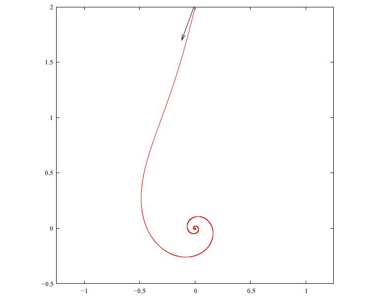
\[ \frac{d r}{d t} = \beta r - r^3 \] \[ \frac{d \theta}{d t} = 1 \]The angle $\theta$ goes around at a constant rate while the radius $r$ does something more interesting. When $\beta \le 0$, you can see that any solution spirals in towards the origin! Or, if it starts at the origin, it stays there. So, we call the origin a "stable equilibrium".
Here's a typical solution for $\beta = -1/4$, drawn as a curve in the $x y$ plane. As time passes, the solution spirals in towards the origin:
The equations are more interesting for $\beta \gt 0$. Then $dr/dt = 0$ whenever
\[ \beta r - r^3 = 0 \]This has two solutions, $r = 0$ and $r = \sqrt{\beta}$. Since $r = 0$ is a solution, the origin is still an equilibrium. But now it's not stable: if $r$ is between $0$ and $\sqrt{\beta}$, we'll have $\beta r - r^3 \gt 0$, so our solution will spiral out, away from the origin and towards the circle $r = \sqrt{\beta}$. So, we say the origin is an "unstable equilibrium". On the other hand, if $r$ starts out bigger than $\sqrt{\beta}$, our solution will spiral in towards that circle.
Here's a picture of two solutions for $\beta = 1$:
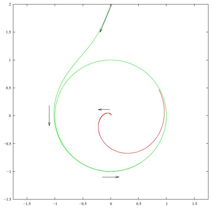
The red solution starts near the origin and spirals out towards the circle $r = \sqrt{\beta}$. The green solution starts outside this circle and spirals in towards it, soon becoming indistinguishable from the circle itself. So, this equation describes a system where $x$ and $y$ quickly settle down to a periodic oscillating behavior.
Since solutions that start anywhere near the circle $r = \sqrt{\beta}$ will keep going round and round getting closer to this circle, it's called a "stable limit cycle".
This is what the Hopf bifurcation is all about! We've got a dynamical system that depends on a parameter, and as we change this parameter, a stable fixed point become unstable, and a stable limit cycle forms around it.
This isn't quite a mathematical definition yet, but it's close enough for now. If you want something a bit more precise, try:
The time between El Niños varies between 3 and 7 years, averaging around 4 years. There can also be two El Niños without an intervening La Niña, or vice versa. One can try to explain this in various ways.
One very simple, general idea to add random noise to whatever differential equation we were using to model the ENSO cycle, obtaining a so-called stochastic differential equation: a differential equation describing a random process. Richard Kleeman discusses this idea in Tim Palmer's book:
Kleeman mentions three general theories for the irregularity of the ENSO. They all involve the idea of separating the weather into "modes" — roughly speaking, different ways that things can oscillate. Some modes are slow and some are fast. The ENSO cycle is defined by the behavior of certain slow modes, but of course these interact with the fast modes. So, there are various options:
Kleeman reviews work on the first option but focuses on the second. The third option is the most complicated, so the pessimist in me suspects that's what's really going on. Still, it's good to start by studying simple models!
How can we get a simple model that illustrates the second option? Simple: take the model we just saw, and add some noise! This idea is discussed in detail here:
This paper is not about the ENSO cycle, but another one, which is often nicknamed the AMO. I would love to talk about it — but not now. Let me just show you the equations for a Hopf bifurcation with noise:
\[ \frac{d x}{d t} = -y + \beta x - x (x^2 + y^2) + \lambda \frac{d W_1}{d t}\] \[ \frac{d y}{d t} = \; x + \beta y - y (x^2 + y^2) + \lambda \frac{d W_2}{d t}\]They're the same as before, but with some new extra terms at the end: that's the noise.
This could easily get a bit technical, but I don't want it to. So, I'll just say some buzzwords and let you click on the links if you want more detail. $W_1$ and $W_2$ are two independent Wiener processes, so they describe Brownian motion in the $x$ and $y$ coordinates. When we differentiate a Wiener process we get white noise. So, we're adding some amount of white noise to the equations we had before, and the number $\lambda$ says precisely how much. That means that $x$ and $y$ are no longer specific functions of time: they're random functions, also known as stochastic processes.
If this were a math course, I'd feel obliged to precisely define all the terms I just dropped on you. But it's not, so I'll just show you some pictures!
If $\beta = 1$ and $\lambda = 0.1$, here are some typical solutions:
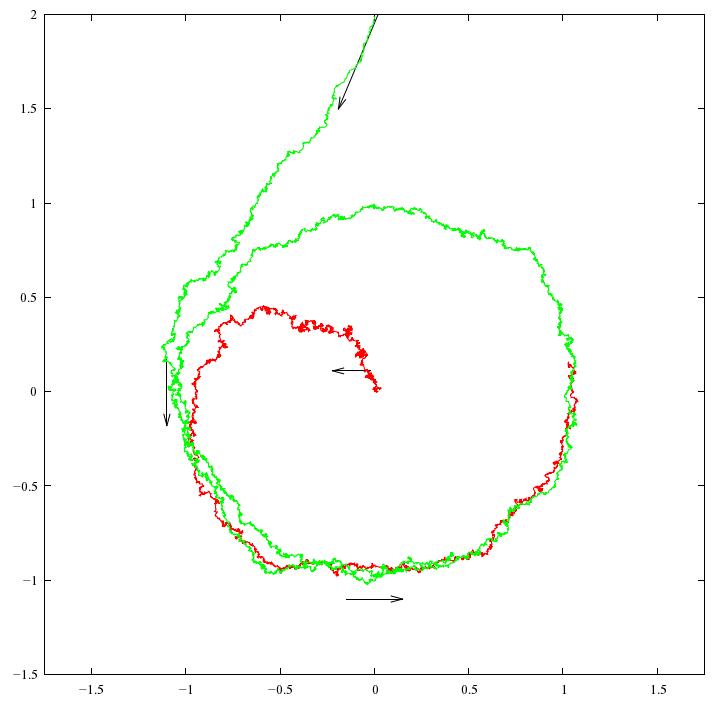
They look similar to the solutions we saw before for $\beta = 1$, but now they have some random wiggles added on.
(You may be wondering what this picture really shows. After all, I said the solutions were random functions of time, not specific functions. But it's tough to draw a "random function". So, to get one of the curves shown above, what Tim did is randomly choose a function according to some rule for computing probabilities, and draw that.)
If we turn up the noise, our solutions get more wiggly. If $\beta = 1$ and $\lambda = 0.3$, they look like this:
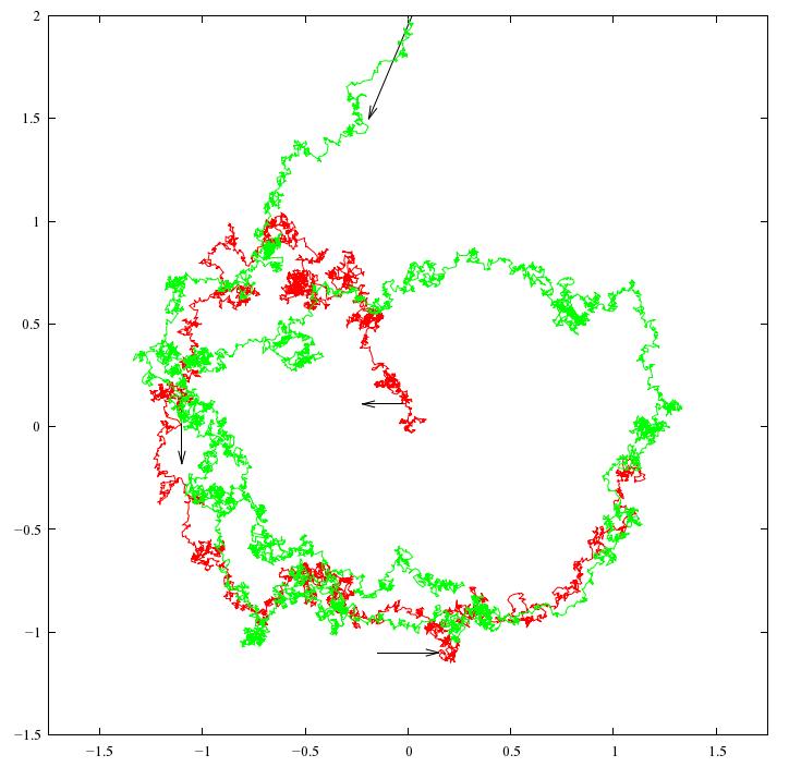
In these examples, $\beta \gt 0$, so we would have a limit cycle if there weren't any noise — and you can see that even with noise, the solutions approximately tend towards the limit cycle. So, we can use an equation of this sort to describe systems that oscillate, but in a somewhat random way.
But now comes the really interesting part! Suppose $\beta \le 0$. Then we've seen that without noise, there's no limit cycle: any solution quickly spirals in towards the origin. But with noise, something a bit different happens. If $\beta = -1/4$ and $\lambda = 0.1$ we get a picture like this:
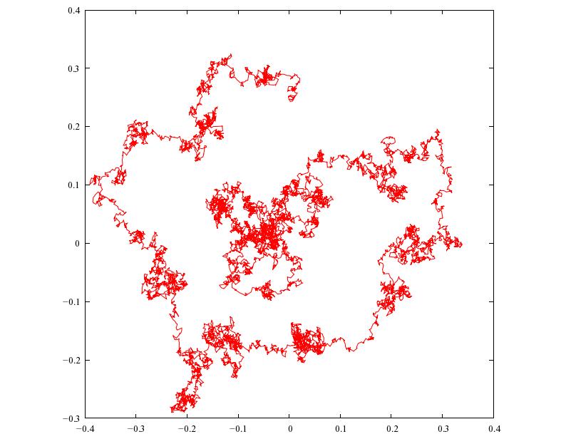
We get irregular oscillations even though there's no limit cycle! Roughly speaking, the noise keeps knocking the solution away from the stable fixed point at $x = y = 0$, so it keeps going round and round, but in an irregular way. It may seem to be spiralling in, but if we waited a bit longer it would get kicked out again.
This is a lot easier to see if we plot just $x$ as a function of $t$. Then we can run our solution for a longer time without the picture becoming a horrible mess:
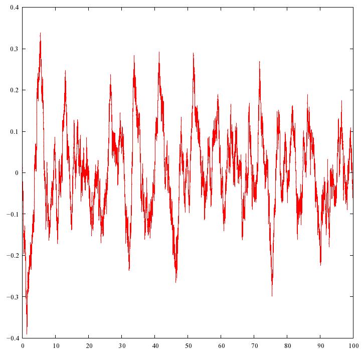
If you compare this with the ENSO cycle, you'll see they look roughly similar:
That's nice. Of course it doesn't prove that a model based on a Hopf bifurcation plus noise is "right" — indeed, we don't really have a model until we've chosen variables for both $x$ and $y$. But it suggests that a model of this sort could be worth studying.
If you want to see how the Hopf bifurcation plus noise is applied to climate cycles, I suggest starting with the paper by Dijkstra, Frankcombe and von der Heydt. If you want to see it applied to the El Niño-Southern Oscillation, start with Section 6.3 of the ENSO theory paper, and then dig into the many references. Here it seems a model with $\beta > 0$ may work best. If so, noise is not required to keep the ENSO cycle going, but it makes the cycle irregular.
To a mathematician like me, what's really interesting is how the addition of noise "smooths out" the Hopf bifurcation. When there's no noise, the qualitative behavior of solutions jumps drastically at $\beta = 0$. For $\beta \gt 0$ we have a stable limit cycle, while for $\beta \le 0$ we have a stable equilibrium. But in the presence of noise, we get irregular cycles not only for $\beta \gt 0$ but also $\beta \le 0$. This is not really surprising, but it suggests a bunch of questions. Such as: what are some quantities we can use to describe the behavior of "irregular cycles", and how do these quantities change as a function of $\lambda$ and $\beta$?
You'll see some answers to this question in Dijkstra, Frankcombe and von der Heydt's paper. However, if you're a mathematician, you'll instantly think of dozens more questions — like, how can I prove what these guys are saying?
If you make any progress, let me know. If you don't know where to start, you might try the Dijkstra et al. paper, and then learn a bit about the Hopf bifurcation, stochastic processes, and stochastic differential equations:
Now, about the Azimuth Code Project. Tim van Beek started it just recently, but the Azimuth Project seems to be attracting people who can program, so I have high hopes for it. Tim wrote:
My main objectives to start the Azimuth Code Project were:
- to have a central repository for the code used for simulations or data analysis on the Azimuth Project,
- to have an online free access repository and make all software open source, to enable anyone to use the software, for example to reproduce the results on the Azimuth Project. Also to show by example that this can and should be done for every scientific publication.
Of less importance is:
- to implement the software with an eye to software engineering principles.
This less important because the world of numerical high performance computing differs significantly from the rest of the software industry: it has special requirements and it is not clear at all which paradigms that are useful for the rest will turn out to be useful here. Nevertheless I'm confident that parts of the scientific community will profit from a closer interaction with software engineering.
So, if you like programming, I hope you'll chat with us and consider joining in! Our next projects involve limit cycles in predator-prey models, stochastic resonance in some theories of the ice ages, and delay differential equations in ENSO models.
And in case you're wondering, the code used for the pictures above is a simple implementation in Java of the Euler scheme, using random number generating algorithms from Numerical Recipes. Pictures were generated with gnuplot.
For more discussion go to my blog, Azimuth.
There are two ways of constructing a software design. One way is to make it so simple that there are obviously no deficiencies. And the other way is to make it so complicated that there are no obvious deficiencies. - C.A.R. Hoare
© 2010 John Baez
baez@math.removethis.ucr.andthis.edu
|
|
|
|