Polyakov's Model

Some people have written saying they enjoy these "Braids and quantization" articles, so I'll keep 'em coming. Some also wrote saying that the best known explanation for the mysterious "fractional quantum Hall effect" involves anyons, and referred me to this paper:

• J. Fröhlich and A. Zee, Large Scale Physics of the Quantum Hall Fluid, Nucl. Phys. B364 (1991), 517-540.

The Hall effect, recall, is fact that if one applies a magnetic field perpendicular to current in a wire, this makes the electrons wnat to veer off to one side (recall the force is proportional to ${\bf v}\mbox{\boldmath$\times$} {\bf B}$), and they do until the increased charge density on that side creates enough electric field to keep more from crowding over to that side. One observes this by measuring the electric field. The "quantum Hall effect" refers to the charming fact that this effect is quantized for a sufficiently good (cold) conductor: as one increases the magnetic field the resulting electric field goes up like a step function; in the right units, the effect takes a jump when the magnetic field is an integer. This effect is reasonably well understood, they say (though I've heard murmurs of discontent occaisionally). I know that Belissard has written nicely about the relationship with noncommutative differential geometry a la Connes. The fractional quantum Hall effect refers to the fact that not only at integers, but also at some fractions, one sees a jump. I will enjoy learning how this could result from fractional (i.e., anyonic) spin and statistics.

Now, though, I feel like rambling on a bit about Polyakov's construction of anyons by adding a Hopf term to the Lagrangian of a certain nonlinear sigma model. This is actually used in the anyonic theory of high-Tc superconductivity, but even if that theory is a bunch of baloney, Polyakov's idea is a charming bit of mathematical-physical speculation. It's a nice introduction to solitons, topological quantum field theories, and Witten's explanation of the new knot polynomials in terms of topological quantum field theories.

Let's say we have two-dimensional magnet. (Ferro- or antiferro- doesn't really matter at the level of vagueness I'll be working at; the high-Tc superconductors are layered crystals that are antiferromagnets in each layer.) We'll just naively assume each atom has a spin which is a unit vector, i.e. a point on $S^2$. And we'll just model the state of the magnet as a spin field, that is, a map from space, ${\bf R}^2$, to $S^2$. (I.e. we're doing a continuum limit: for antiferromagnets we flip over the spin of every other atom (in our model) to get a nice continuous map from ${\bf R}^2$ to $S^2$.) Let's assume that all the spins are lined up at spatial infinity. Thus we can add a point at infinity to ${\bf R}^2$ (getting a sphere $S^2$) and describe the state of our magnet as a map from $S^2$ to $S^2$. Physicists like to use the delightfully uninformative term "nonlinear sigma model" to describe a field theory in which the field is a map from one manifold (e.g. $S^2$) to another (e.g. $S^2$) -- a generalization of the usual vector or tensor field. So we've got ourselves a simple nonlinear sigma model to describe the 2d magnet. I should tell you the Lagrangian but I'm carefully avoiding any equations, so I'll just say (for those in the know) that it's the one that gives harmonic maps.

Now, maps from $S^2$ to $S^2$ come in various homotopy classes, that is, different maps from $S^2$ to $S^2$ may not be able to be continuously deformed into each other. It is a little hard for me to draw these things, but they really aren't hard to visualize with some work. Just as the homotopy classes of maps from $S^1$ to itself are indexed by an integer, the winding number, so are the maps from $S^2$ to itself: there's a kind of "winding number" that counts (with sign) how many times you've wrapped the sphere over itself. These twists in the field act sort of like localized particles (for a lower-dimensional analogy imagine them as twists in a ribbon) and are called topological solitons. For physicists, the "winding number" I mentioned above is called the soliton number. It acts like a conserved charge. One can start with a field configuration with zero soliton number - all spins lined straight up - and then have a soliton-antisoliton pair form, move around, and then annihilate, for example. Note that if we track the birth and death of soliton-antisoliton pairs over time by drawing their worldlines, we get a link! This is where knots and braids sneak into the picture:

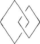
In this picture time goes up the page, and we see first one pair formed, then another, then they move around each other and then they annihilate. We have a link with linking number 1 (let's say -- the sign actually depends on a right-hand rule, but since I'm left-handed I object to using the usual right-hand rule).

Polyakov's trick was to add a term to the Lagrangian which equals a constant $\theta$ times the linking number. It's a bit more technical so before describing how he gets a local expression for this term I'll just say what its effect is on the physics. Classically, it has no effect whatsoever! Since a small variation in the field configuation doesn't change the linking number (which after all is a topological invariant), the Euler-Lagrange equations (which come from differentiating the Lagrangian) don't notice this term at all. Quantum mechanically, however, one doesn't just look for an extremum of the action. Instead one forms a path integral a la Feynman, integrating $\exp(i {\rm Action})$ over all histories. So if two histories have different linking numbers, their contribution to the integral will differ by a phase. For example, the configuration above has the exact same action as this one:

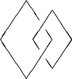
by symmetry, except that the first, "right-handed", history has linking number $1$, while the second, "left-handed" one has linking number $-$1. Thus the first will appear in the path integral with a factor of $e^{i\theta}$, while the second will appear with a factor of $e^{-i\theta}$. Thus if one soliton goes around another we get a phase factor, so -- here the reader needs a bit of faith -- they act like anyons.

Now let me describe Polyakov's term in the Lagrangian in a bit more detail. Here I'll allow myself to be a tad more technical. Let us assume that (as in the pictures above) we are considering histories which begin and end with all spins lined up. Thus our map from spacetime (2d space, 1d time) to $S^2$ may be regarded as a map from $S^3$ to $S^2$, using the old "point at infinity" trick again. The homotopy classes of maps from $S^3$ to $S^2$ are also indexed by an integer, this being called the Hopf invariant. The first way to calculate the Hopf invariant shows why Polyakov uses it as an extra term in the Lagrangian. Take a map from $S^3$ to $S^2$. By Sard's theorem almost every point in $S^2$ will have as its inverse image in $S^3$ a collection of nonintersecting closed curves (i.e., a link). The Hopf invariant may be calculated as follows: take two such points in $S^2$ and call their inverse images in $S^3$, $L$ and $L'$. The Hopf invariant is the linking number ${\rm link}(L,L')$ (which doesn't depend on which points you picked). To see how this relates to the story above, take two nearby points in $S^2$ and draw an arc between them. The inverse image of this arc in $S^3$ is a "ribbon" or "framed link," and the Hopf invariant, ${\rm link}(L,L')$, is also called the "self-linking number" of the framed link, since it includes information about how the ribbon twists, as well as how it links itself when it has more than one connected component. Physically, the contribution to the Hopf invariant due to ribbon twisting is interpreted as due to the rotation of individual anyons. Since spin as well as statistics contributes to the phase $\exp(i {\rm Action})$, to be precise one must model the anyon trajectories not by a link in spacetime, but by a framed link, which keeps track of how they rotate.

The second way to calculate the Hopf invariant shows how to write it down as an integral over $S^3$ of a local expression (Lagrangian density). Take the volume form on $S^2$ and pull it back to $S^3$ by our map. We now have a closed 2-form on $S^3$ so we can write it as $dA$ for some 1-form. Now integrate $A\wedge dA$ over $S^2$ and divide by something like $4\pi$. This is the Hopf invariant! I leave it as an easy exercise to show that it didn't depend on our choice of $A$, and as a slightly harder exercise to show that it really is a diffeomorphism invariant, and as a harder exercise to show that this definition of the Hopf invariant agrees with the linking number one. (For more info read Bott and Tu's Differential Forms and Algebraic Topology.)

Note that the freedom of choice of $A$ here is none other than what physicists call "gauge freedom." What we have here, in other words, is a gauge theory with a diffeomorphism invariant Lagrangian. (That is, if we keep the Hopf term and drop the harmonic action.) Such theories give boring classical dynamics, because the action is constant on each connected component of the path space. (Or, in physics lingo, the Lagrangian is a total divergence.) But they can give nontrivial dynamics after quantization, because of phase effects. In fact, the simplest example of this sort of deal is the Bohm-Aharonov effect. The particle can go around an obstacle in either of two ways so the path space consists of two components. Classically, a term in the action that is constant on each component doesn't do anything. But quantum-mechanically it leads to interference due to a shift of phase.

These days the ultrasophisticated mathematical physicists and topologists love talking to each other about "topological quantum field theories" in which the Lagrangian is a diffeomorphism invariant. The term with action equal to the integral of $A\wedge dA$ is called the "$U(1)$ Chern-Simons theory", because a 1-form may be regarded as a connection on a $U(1)$ bundle. This is a very simple theory; the more interesting ones use nonabelian gauge groups. Witten showed (in his rough-and-ready manner) that just as the linking number is related to the $U(1)$ Chern-Simons theory, the Jones polynomial is related to the $SU(2)$ Chern-Simons theory. (Many people have been trying to make this more rigorous. Right now my friend Scott Axelrod is working with Singer on the perturbation theory for Chern-Simons theory, which should make the story quite precise.)

© 1992 John Baez
baez@math.removethis.ucr.andthis.edu

home