January 7, 2013

Lyapunov Functions for Complex-Balanced Systems

Manoj Gopalkrishnan

A few weeks back, I promised to tell you more about a long-standing open problem in reaction networks, the 'global attractor conjecture'. I am not going to quite get there today, but we shall take one step in that direction.

Today's plan is to help you make friends with a very useful function we will call the 'free energy' which comes up all the time in the study of chemical reaction networks. We will see that for complex-balanced systems, the free energy function decreases along trajectories of the rate equation. I'm going to explain this statement, and give you most of the proof!

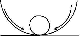
The point of doing all this work is that we will then be able to invoke Lyapunov's theorem which implies stability of the dynamics. In Greek mythology, Sisyphus was cursed to roll a boulder up a hill only to have it roll down again, so that he had to keep repeating the task for all eternity. When I think of an unstable equilibrium, I imagine a boulder delicately balanced on top of a hill, which will fall off if given the slightest push:

or, more abstractly:

On the other hand, I picture a stable equilibrium as a pebble at the very bottom of a hill. Whichever way a perturbation takes it is up, so it will roll down again to the bottom:

Lyapunov's theorem guarantees stability provided we can exhibit a nice enough function $V$ that decreases along trajectories. 'Nice enough' means that, viewing $V$ as a height function for the hill, the equilibrium configuration should be at the bottom, and every direction from there should be up. If Sisyphus had dug a pit at the top of the hill for the boulder to rest in, Lyapunov's theorem would have applied, and he could have gone home to rest. The moral of the story is that it pays to learn dynamical systems theory!

Because of the connection to Lyapunov's theorem, such functions that decrease along trajectories are also called Lyapunov functions. A similar situation is seen in Boltzmann's H-theorem, and hence such functions are sometimes called H-functions by physicists.

Another reason for me to talk about these ideas now is that I have posted a new article on the arXiv:

• Manoj Gopalkrishnan, On the Lyapunov function for complex-balanced mass-action systems.

The free energy function in chemical reaction networks goes back at least to 1972, to this paper:

• Friedrich Horn and Roy Jackson, General mass action kinetics, Arch. Rational Mech. Analysis 49 (1972), 81–116.

Many of us credit Horn and Jackson's paper with starting the mathematical study of reaction networks. My paper is an exposition of the main result of Horn and Jackson, with a shorter and simpler proof. The gain comes because Horn and Jackson proved all their results from scratch, whereas I'm using some easy results from graph theory, and the log-sum inequality.

We shall be talking about reaction networks. Remember the idea from the network theory series. We have a set $S$ whose elements are called species, for example

A complex is a vector of natural numbers saying how many items of each species we have. For example, we could have a complex $(2,3,1).$ But chemists would usually write this as

A reaction network is a set $S$ of species and a set $T$ of transitions or reactions, where each transition $\tau \in T$ goes from some complex $m(\tau)$ to some complex $n(\tau).$ For example, we could have a transition $\tau$ with

and

In this situation chemists usually write

but we want names like $\tau$ for our transitions, so we might write

or

As John explained in Part 3 of the network theory series, chemists like to work with a vector of nonnegative real numbers $x(t)$ saying the concentration of each species at time $t.$ If we know a rate constant $r(\tau) > 0$ for each transition $\tau$, we can write down an equation saying how these concentrations change with time:

This is called the rate equation. It's really a system of ODEs describing how the concentration of each species change with time. Here an expression like $x^m$ is shorthand for the monomial ${x_1}^{m_1} \cdots {x_k}^{m_k}$. John and Brendan talked about complex balance in Part 9. I'm going to recall this definition, from a slightly different point of view that will be helpful for the result we are trying to prove.

We can draw a reaction network as a graph! The vertices of this graph are all the complexes $m(\tau), n(\tau)$ where $\tau \in T$. The edges are all the transitions $\tau\in T$. We think of each edge $\tau$ as directed, going from $m(\tau)$ to $n(\tau)$.

We will call the map that sends each transition $\tau$ to the positive real number $r(\tau) x^{m(\tau)}$ the flow $f_x(\tau)$ on this graph. The rate equation can be rewritten very simply in terms of this flow as:

where the right-hand side is now a linear expression in the flow $f_x$.

Flows of water, or electric current, obey a version of Kirchhoff's current law. Such flows are called conservative flows. The following two lemmas from graph theory are immediate for conservative flows:

Lemma 1. If f is a conservative flow then the net flow across every cut is zero.

A cut is a way of chopping the graph in two, like this:

It's easy to prove Lemma 1 by induction, moving one vertex across the cut at a time.

Lemma 2. If a conservative flow exists then every edge $\tau\in T$ is part of a directed cycle.

Why is Lemma 2 true? Suppose there exists an edge $\tau : m \to n$ that is not part of any directed cycle. We will exhibit a cut with non-zero net flow. By Lemma 1, this will imply that the flow is not conservative.

One side of the cut will consist of all vertices from which $m$ is reachable by a directed path in the reaction network. The other side of the cut contains at least $n$, since $m$ is not reachable from $n$, by the assumption that $\tau$ is not part of a directed cycle. There is flow going from left to right of the cut, across the transition $\tau$. Since there can be no flow coming back, this cut has nonzero net flow, and we're done.     ▮

Now, back to the rate equation! We can ask if the flow $f_x$ is conservative. That is, we can ask if, for every complex $n$:

In words, we are asking if the sum of the flow through all transitions coming in to $n$ equals the sum of the flow through all transitions going out of $n$. If this condition is satisfied at a vector of concentrations $x = \alpha$, so that the flow $f_\alpha$ is conservative, then we call $\alpha$ a point of complex balance. If in addition, every component of $\alpha$ is strictly positive, then we say that the system is complex balanced.

Clearly if $\alpha$ is a point of complex balance, it's an equilibrium solution of the rate equation. In other words, $x(t) = \alpha$ is a solution of the rate equation, where $x(t)$ never changes.

I'm using 'equilibrium' the way mathematicians do. But I should warn you that chemists use 'equilibrium' to mean something more than merely a solution that doesn't change with time. They often also mean it's a point of complex balance, or even more. People actually get into arguments about this at conferences.

Complex balance implies more than mere equilibrium. For starters, if a reaction network is such that every edge belongs to a directed cycle, then one says that the reaction network is weakly reversible. So Lemmas 1 and 2 establish that complex-balanced systems must be weakly reversible!

From here on, we fix a complex-balanced system, with $\alpha$ a strictly positive point of complex balance.

Definition. The free energy function is the function

where the sum is over all species in $S$.

The whole point of defining the function this way is because it is the unique function, up to an additive constant, whose partial derivative with respect to $x_s$ is $\log x_s/\alpha_s$. This is important enough that we write it as a lemma. To state it in a pithy way, it is helpful to introduce vector notation for division and logarithms. If $x$ and $y$ are two vectors, we will understand $x/y$ to mean the vector $z$ such that $z_s = x_s/ y_s$ coordinate-wise. Similarly $\log x$ is defined in a coordinate-wise sense as the vector with coordinates $(\log x)_s = \log x_s$.

Lemma 3. The gradient $\nabla g_\alpha(x)$ of $g_\alpha(x)$ equals $\log(x/\alpha)$.

We're ready to state our main theorem!

Theorem. Fix a trajectory $x(t)$ of the rate equation. Then $g_\alpha(x(t))$ is a decreasing function of time $t$. Further, it is strictly decreasing unless $x(t)$ is an equilibrium solution of the rate equation.

I find precise mathematical statements reassuring. You can often make up your mind about the truth value from a few examples. Very often, though not always, a few well-chosen examples are all you need to get the general idea for the proof. Such is the case for the above theorem. There are three key examples: the two-cycle, the three-cycle, and the figure-eight.

The two-cycle. The two-cycle is this reaction network:

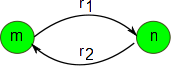
It has two complexes $m$ and $n$ and two transitions $\tau_1 = m\to n$ and $\tau_2 = n\to m$, with rates $r_1 = r(\tau_1)$ and $r_2 = r(\tau_2)$ respectively.

Fix a solution $x(t)$ of the rate equation. Then the flow from $m$ to $n$ equals $r_1 x^m$ and the backward flow equals $r_2 x^n$. The condition for $f_\alpha$ to be a conservative flow requires that $f_\alpha = r_1 \alpha^m = r_2 \alpha^n$. This is one binomial equation in at least one variable, and clearly has a solution in the positive reals. We have just shown that every two-cycle is complex balanced.

The derivative $d g_\alpha(x(t))/d t$ can now be computed by the chain rule, using Lemma 3. It works out to $f_\alpha$ times

This is never positive, and it's zero if and only if

Why is this? Simply because the logarithm of something greater than 1 is positive, while the log of something less than 1 is negative, so that the sign of $(x/\alpha)^m - (x/\alpha)^n$ is always opposite the sign of $\log \frac{(x/\alpha)^n}{(x/\alpha)^m}$. We have verified our theorem for this example.

(Note that $(x/\alpha)^m = (x/\alpha)^n$ occurs when $x = \alpha$, but also at other points: in this example, there is a whole hypersurface consisting of points of complex balance.)

In fact, this simple calculation achieves much more.

Definition. A reaction network is reversible if for every transition $\tau : m \to n$ there is a transition $\tau' : m \to n$ going back, called the reverse of $\tau$. Suppose we have a reversible reaction network and a vector of concentrations $\alpha$ such that the flow along each edge equals that along the edge going back:

whenever $\tau'$ is the reverse $\tau$. Then we say the reaction network is detailed balanced, and $\alpha$ is a point of detailed balance.

For a detailed-balanced system, the time derivative of $g_\alpha$ is a sum over the contributions of pairs consisting of an edge and its reverse. Hence, the two-cycle calculation shows that the theorem holds for all detailed balanced systems!

This linearity trick is going to prove very valuable. It will allow us to treat the general case of complex balanced systems one cycle at a time. The proof for a single cycle is essentially contained in the example of a three-cycle, which we treat next:

The three-cycle. The three-cycle is this reaction network:

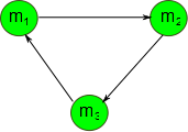
We assume that the system is complex balanced, so that

Let us call this nonnegative number $f_\alpha$. A small calculation employing the chain rule shows that $d g_\alpha(x(t))/d t$ equals $f_\alpha$ times

We need to think about the sign of this quantity:

Lemma 3. Let $a,b,c$ be positive numbers. Then $a \log b/a + b\log c/b + c\log a/c$ is less than or equal to zero, with equality precisely when $a=b=c$.

The proof is a direct application of the log sum inequality. In fact, this holds not just for three numbers, but for any finite list of numbers. Indeed, that is precisely how one obtains the proof for cycles of arbitrary length. Even the two-cycle proof is a special case! If you are wondering how the log sum inequality is proved, it is an application of Jensen's inequality, that workhorse of convex analysis.

The three-cycle calculation extends to a proof for the theorem so long as there is no directed edge that is shared between two directed cycles. When there are such edges, we need to argue that the flows $f_\alpha$ and $f_x$ can be split between the cycles sharing that edge in a consistent manner, so that the cycles can be analyzed independently. We will need the following simple lemma about conservative flows from graph theory. We will apply this lemma to the flow $f_\alpha$.

Lemma 4. Let $f$ be a conservative flow on a graph $G$. Then there exist directed cycles $C_1, C_2,\dots, C_k$ in $G$, and nonnegative real 'flows' $f_1,f_2,\dots,f_k \in [0,\infty]$ such that for each directed edge $e$ in $G$, the flow $f(e)$ equals the sum of $f_i$ over $i$ such the cycle $C_i$ contains the edge $e$.

Intuitively, this lemma says that conservative flows come from constant flows on the directed cycles of the graph. How does one show this lemma? I'm sure there are several proofs, and I hope some of you can share some of the really neat ones with me. The one I employed was algorithmic. The idea is to pick a cycle, any cycle, and subtract the maximum constant flow that this cycle allows, and repeat. This is most easily understood by looking at the example of the figure-eight:

The figure-eight. This reaction network consists of two three-cycles sharing an edge:

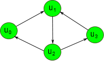
Here's the proof for Lemma 4. Let $f$ be a conservative flow on this graph. We want to exhibit cycles and flows on this graph according to Lemma 4. We arbitrarily pick any cycle in the graph. For example, in the figure-eight, suppose we pick the cycle $u_0\to u_1\to u_2\to u_0$. We pick an edge in this cycle on which the flow is minimum. In this case, $f(u_0\to u_1) = f(u_2\to u_0)$ is the minimum. We define a remainder flow by subtracting from $f$ this constant flow which was restricted to one cycle. So the remainder flow is the same as $latexf$ on edges that don't belong to the picked cycle. For edges that belong to the cycle, the remainder flow is $f$ minus the minimum of $f$ on this cycle. We observe that this remainder flow satisfies the conditions of Lemma 4 on a graph with strictly fewer edges. Continuing in this way, since the lemma is trivially true for the empty graph, we are done by infinite descent.

Now that we know how to split the flow $f_\alpha$ across cycles, we can figure out how to split the rates across the different cycles. This will tell us how to split the flow $f_x$ across cycles. Again, this is best illustrated by an example.

The figure-eight. Again, this reaction network looks like

Suppose as in Lemma 4, we obtain the cycles

with constant flow $f_\alpha^1$

and

with constant flow $f_\alpha^2$ such that

Here's the picture:

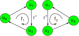
Then we obtain rates $r^1(u_1\to u_2)$ and $r^2(u_1\to u_2)$ by solving the equations

Using these rates, we can define non-constant flows $f^1_x$ on $C_1$ and $f^2_x$ on $C_2$ by the usual formulas:

and similarly for $f^2_x$. In particular, this gives us

and similarly for $f^2_x$.

Using this, we obtain the proof of the Theorem! The time derivative of $g_\alpha$ along a trajectory has a contribution from each cycle $C$ as in Lemma 4, where each cycle is treated as a separate system with the new rates $r^C$, and the new flows $f^C_\alpha$ and $f^C_x$. So, we've reduced the problem to the case of a cycle, which we've already done.

Let's review what happened. The time derivative of the function $g_\alpha$ has a very nice form, which is linear in the flow $f_x$. The reaction network can be broken up into cycles. The conservative flow $f_\alpha$ for a complex balanced system can be split into conservative flows on cycles by Lemma 4. This informs us how to split the non-conservative flow $f_x$ across cycles. By linearity of the time derivative, we can separately treat the case for every cycle. For each cycle, we get an expression to which the log sum inequality applies, giving us the final result that $g_\alpha$ decreases along trajectories of the rate equation.

You can also read comments on Azimuth, and make your own comments or ask questions there!

© 2013 Manoj Gopalkrishan
baez@math.removethis.ucr.andthis.edu
home