

|
|
|
|
H + OH → H2O
and population biology:
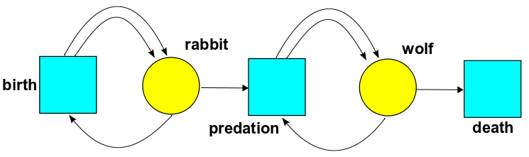
amoeba → amoeba + amoeba
and the study of infectious diseases:
infected + susceptible → infected + infected
and many other situations.
A "stochastic" Petri net says the rate at which each transition occurs. We can think of these transitions as occurring randomly at a certain rate—and then we get a stochastic process described by something called the "master equation". But for starters, we've been thinking about the limit where there are very many things in each state. Then the randomness washes out, and the expected number of things in each state changes deterministically in a manner described by the "rate equation".
It's time to explain the general recipe for getting this rate equation! It looks complicated at first glance, so I'll briefly state it, then illustrate it with tons of examples, and then state it again.
One nice thing about stochastic Petri nets is that they let you dabble in many sciences. Last time we got a tiny taste of how they show up in population biology. This time we'll look at chemistry and models of infectious diseases. I won't dig very deep, but take my word for it: you can do a lot with stochastic Petri nets in these subjects! I'll give some references in case you want to learn more.
Here's the recipe, really quickly:
A stochastic Petri net has a set of states and a set of transitions. Let's concentrate our attention on a particular transition. Then the $ i$th state will appear $ m_i$ times as the input to that transition, and $ n_i$ times as the output. Our transition also has a reaction rate $ 0 < r < \infty$.
The rate equation answers this question:
$$ \frac{d x_i}{d t} = ??? $$
where $ x_i(t)$ is the number of things in the $ i$th state at time $ t$. The answer is a sum of terms, one for each transition. Each term works the same way. For the transition we're looking at, it's
$$ r (n_i - m_i) x_1^{m_1} \cdots x_k^{m_k} $$
The factor of $ (n_i - m_i)$ shows up because our transition destroys $ m_i$ things in the $ i$th state and creates $ n_i$ of them. The big product over all states, $ x_1^{m_1} \cdots x_k^{m_k} $, shows up because our transition occurs at a rate proportional to the product of the numbers of things it takes as inputs. The constant of proportionality is the reaction rate $r$.
But let's do an example. Here's a naive model for the formation of water from atomic hydrogen and oxygen:
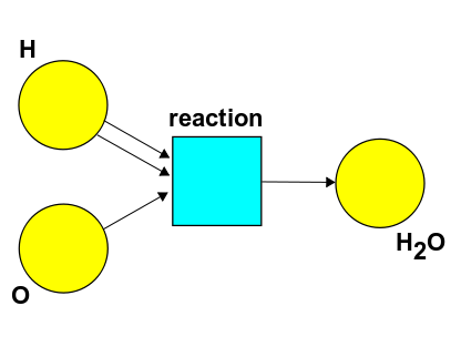
This Petri net has just one transition: two hydrogen atoms and an oxygen atom collide simultaneously and form a molecule of water. That's not really how it goes... but what if it were? Let's use $ [\mathrm{H}]$ for the number of hydrogen atoms, and so on, and let the reaction rate be $ \alpha$. Then we get this rate equation:
$$ \begin{array}{ccl} \displaystyle{ \frac{d [\mathrm{H}]}{d t}} &=& - 2 \alpha [\mathrm{H}]^2 [\mathrm{O}] \\ \quad \\ \displaystyle{ \frac{d [\mathrm{O}]}{d t}} &=& - \alpha [\mathrm{H}]^2 [\mathrm{O}] \\ \quad \\ \displaystyle{ \frac{d [\mathrm{H}_2\mathrm{O}]}{d t}} &=& \alpha [\mathrm{H}]^2 [\mathrm{O}] \end{array} $$
See how it works? The reaction occurs at a rate proportional to the product of the numbers of things that appear as inputs: two H's and one O. The constant of proportionality is the rate constant $\alpha$. So, the reaction occurs at a rate equal to $ \alpha [\mathrm{H}]^2 [\mathrm{O}] $. Then:
• Since two hydrogen atoms get used up in this reaction, we get a factor of $ -2$ in the first equation.
• Since one oxygen atom gets used up, we get a factor of $ -1$ in the second equation.
• Since one water molecule is formed, we get a factor of $ +1$ in the third equation.
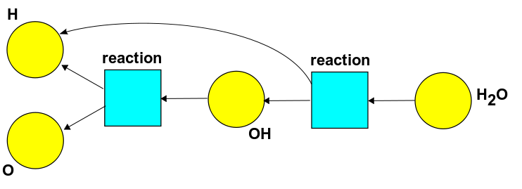
Let me do another example, just so chemists don't think I'm an absolute ninny. Chemical reactions rarely proceed by having three things collide simultaneously—it's too unlikely. So, for the formation of water from atomic hydrogen and oxygen, there will typically be an intermediate step. Maybe something like this:
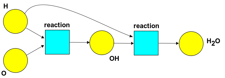
Here OH is called a 'hydroxyl radical'. I'm not sure this is the most likely pathway, but never mind—it's a good excuse to work out another rate equation. If the first reaction has rate constant $\alpha$ and the second has rate constant $\beta$, here's what we get:
$$ \begin{array}{ccl} \displaystyle{ \frac{d [\mathrm{H}]}{d t} } &=& - \alpha [\mathrm{H}] [\mathrm{O}] - \beta [\mathrm{H}] [\mathrm{OH}] \\ \quad \\ \displaystyle{\frac{d [\mathrm{OH}]}{d t} } &=& \alpha [\mathrm{H}] [\mathrm{O}] - \beta [\mathrm{H}] [\mathrm{OH}] \\ \quad \\ \displaystyle{\frac{d [\mathrm{O}]}{d t} } &=& - \alpha [\mathrm{H}] [\mathrm{O}] \\ \quad \\ \displaystyle{\frac{d [\mathrm{H}_2\mathrm{O}]}{d t} } &=& \beta [\mathrm{H}] [\mathrm{OH}] \end{array} $$
See how it works? Each reaction occurs at a rate proportional to the product of the numbers of things that appear as inputs. We get minus signs when a reaction destroys one thing of a given kind, and plus signs when it creates one. We don't get factors of 2 as we did last time, because now no reaction creates or destroys two of anything.
In chemistry every reaction comes with a reverse reaction. So, if hydrogen and oxygen atoms can combine to form water, a water molecule can also 'dissociate' into hydrogen and oxygen atoms. The rate constants for the reverse reaction can be different than for the original reaction... and all these rate constants depend on the temperature. At room temperature, the rate constant for hydrogen and oxygen to form water is a lot higher than the rate constant for the reverse reaction. That's why we see a lot of water, and not many lone hydrogen or oxygen atoms. But at sufficiently high temperatures, the rate constants change, and water molecules become more eager to dissociate.
Calculating these rate constants is a big subject. I'm just starting to read this book, which looked like the easiest one on the library shelf:
• S. R. Logan, Chemical Reaction Kinetics, Longman, Essex, 1996.
But let's not delve into these mysteries today. Let's just take our naive Petri net for the formation of water and turn around all the arrows, to get the reverse reaction:
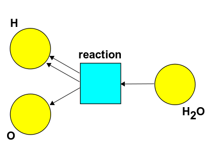
If the reaction rate is $\alpha$, here's the rate equation: $$ \begin{array}{ccl} \displaystyle{\frac{d [\mathrm{H}]}{d t}} &=& 2 \alpha [\mathrm{H}_2\mathrm{O}] \\ \quad \\ \displaystyle{\frac{d [\mathrm{O}]}{d t}} &=& \alpha [\mathrm{H}_2 \mathrm{O}] \\ \quad \\ \displaystyle{\frac{d [\mathrm{H}_2\mathrm{O}]}{d t}} &=& - \alpha [\mathrm{H}_2 \mathrm{O}] \end{array} $$
See how it works? The reaction occurs at a rate proportional to $ [\mathrm{H}_2\mathrm{O}]$, since it has just a single water molecule as input. That's where the $ \alpha [\mathrm{H}_2\mathrm{O}]$ comes from. Then:
• Since two hydrogen atoms get formed in this reaction, we get a factor of +2 in the first equation.
• Since one oxygen atom gets formed, we get a factor of +1 in the second equation.
• Since one water molecule gets used up, we get a factor of +1 in the third equation.
Of course, we can also look at the reverse of the more realistic reaction involving a hydroxyl radical as an intermediate. Again, we just turn around the arrows in the Petri net we had:
Now the rate equation looks like this:
$$ \begin{array}{ccl} \displaystyle{\frac{d [\mathrm{H}]}{d t}} &=& + \alpha [\mathrm{OH}] + \beta [\mathrm{H}_2\mathrm{O}] \\ \quad \\ \displaystyle{\frac{d [\mathrm{OH}]}{d t}} &=& - \alpha [\mathrm{OH}] + \beta [\mathrm{H}_2 \mathrm{O}] \\ \quad \\ \displaystyle{\frac{d [\mathrm{O}]}{d t}} &=& + \alpha [\mathrm{OH}] \\ \quad \\ \displaystyle{\frac{d [\mathrm{H}_2\mathrm{O}]}{d t}} &=& - \beta [\mathrm{H}_2\mathrm{O}] \end{array} $$
Do you see why? Test your understanding of the general recipe.
By the way: if you're a category theorist, when I said "turn around all the arrows" you probably thought "opposite category". And you'd be right! A Petri net is just a way of presenting of a strict symmetric monoidal category that's freely generated by some objects (the states) and some morphisms (the transitions). When we turn around all the arrows in our Petri net, we're getting a presentation of the opposite symmetric monoidal category. For more details, try:
• Vladimiro Sassone, On the category of Petri net computations, 6th International Conference on Theory and Practice of Software Development, Proceedings of TAPSOFT '95, Lecture Notes in Computer Science 915, Springer, Berlin, pp. 334-348.
After I explain how stochastic Petri nets are related to quantum field theory, I hope to say more about this category theory business. But if you don't understand it, don't worry about it now—let's do a few more examples.
The SI model is an extremely simple model of an infectious disease. We can describe it using this Petri net:
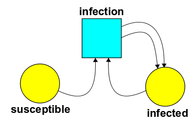
There are two states: susceptible and infected. And there's a transition called infection, where an infected person meets a susceptible person and infects them.
Suppose $S$ is the number of susceptible people and $I$ the number of infected ones. If the rate constant for infection is $\beta$, the rate equation is $$ \begin{array}{ccl} \displaystyle{\frac{d S}{d t}} &=& - \beta S I \\ \quad \\ \displaystyle{\frac{d I}{d t}} &=& \beta S I \end{array} $$
Do you see why?
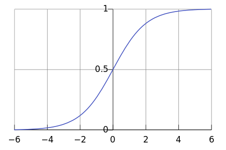
By the way, it's easy to solve these equations exactly. The total number of people doesn't change, so $ S + I$ is a conserved quantity. Use this to get rid of one of the variables. You'll get a version of the famous logistic equation, so the fraction of people infected must grow sort of like this:
Puzzle 1. Is there a stochastic Petri net with just one state whose rate equation is the logistic equation:
$$ \frac{d P}{d t} = \alpha P - \beta P^2 \; ?$$
The SI model is just a warmup for the more interesting SIR model, which was invented by Kermack and McKendrick in 1927:
• W. O. Kermack and A. G. McKendrick, A Contribution to the mathematical theory of epidemics, Proc. Roy. Soc. Lond. A 115 (1927), 700-721.
The SIR model has an extra state, called resistant, and an extra transition, called recovery, where an infected person gets better and develops resistance to the disease:
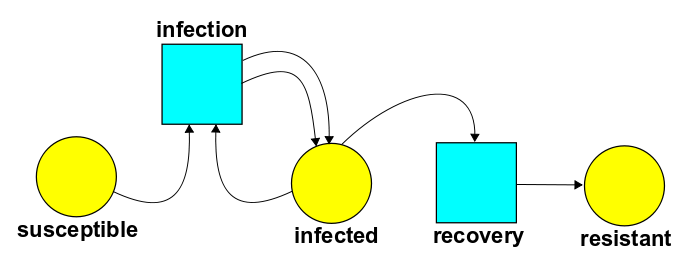
If the rate constant for infection is $ \beta$ and the rate constant for recovery is $ \alpha$, the rate equation for this stochastic Petri net is: $$ \begin{array}{ccl} \frac{d S}{d t} &=& - \beta S I \\ \\ \frac{d I}{d t} &=& \beta S I - \alpha I \\ \\ \frac{d R}{d t} &=& \alpha I \end{array} $$
See why?
I don't know a 'closed-form' solution to these equations. But Kermack and McKendrick found an approximate solution in their original paper. They used this to model the death rate from bubonic plague during an outbreak in Bombay, and got pretty good agreement. Nowadays, of course, we can solve these equations numerically on the computer.
There's an even more interesting model of infectious disease called the SIRS model. This has one more transition, called losing resistance, where a resistant person can go back to being susceptible. Here's the Petri net:
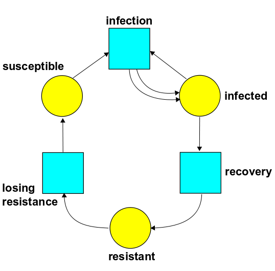
Puzzle 2. If the rate constants for recovery, infection and loss of resistance are $ \alpha, \beta,$ and $ \gamma$, write down the rate equations for this stochastic Petri net.
In the SIRS model we see something new: cyclic behavior! Say you start with a few infected people and a lot of susceptible ones. Then lots of people get infected... then lots get resistant... and then, much later, if you set the rate constants right, they lose their resistance and they're ready to get sick all over again! You can sort of see it from the Petri net, which looks like a cycle.
I learned about the SI, SIR and SIRS models from this great book:
• Marc Mangel, The Theoretical Biologist's Toolbox: Quantitative Methods for Ecology and Evolutionary Biology, Cambridge U. Press, Cambridge, 2006.
For more models of this type, see:
• Compartmental models in epidemiology, Wikipedia.
A 'compartmental model' is closely related to a stochastic Petri net, but beware: the pictures in this article are not really Petri nets!
Now let me remind you of the general recipe and polish it up a bit. So, suppose we have a stochastic Petri net with $ k$ states. Let $ x_i$ be the number of things in the $ i$th state. Then the rate equation looks like:
$$ \frac{d x_i}{d t} = ??? $$
It's really a bunch of equations, one for each $ 1 \le i \le k$. But what is the right-hand side?
The right-hand side is a sum of terms, one for each transition in our Petri net. So, let's assume our Petri net has just one transition! (If there are more, consider one at a time, and add up the results.)
Suppose the $ i$th state appears as input to this transition $m_i$ times, and as output $n_i$ times. Then the rate equation is $$ \frac{d x_i}{d t} = r (n_i - m_i) x_1^{m_1} \cdots x_k^{m_k} $$
where $r$ is the rate constant for this transition.
That's really all there is to it! But subscripts make my eyes hurt more and more as I get older—this is the real reason for using index-free notation, despite any sophisticated rationales you may have heard—so let's define a vector
$$ x = (x_1, \dots , x_k) $$
that keeps track of how many things there are in each state. Similarly let's make up an input vector:
$$ m = (m_1, \dots, m_k) $$
and an output vector:
$$ n = (n_1, \dots, n_k) $$
for our transition. And a bit more unconventionally, let's define $$ x^m = x_1^{m_1} \cdots x_k^{m_k} $$
Then we can write the rate equation for a single transition as
$$ \frac{d x}{d t} = r (n-m) x^m $$
This looks a lot nicer! Any equation with more than 20 symbols is too ugly for me to enjoy.
Indeed, this emboldens me to consider a general stochastic Petri net with lots of transitions, each with their own rate constant. Let's write $ T$ for the set of transitions and $ r(\tau)$ for the rate constant of the transition $ \tau \in T$. Let $ n(\tau)$ and $ m(\tau)$ be the input and output vectors of the transition $ \tau$. Then the rate equation for our stochastic Petri net is
$$ \frac{d x}{d t} = \sum_{\tau \in T} r(\tau) (n(\tau) - m(\tau)) x^{m(\tau)} $$
That's the fully general recipe in a nutshell. I'm not sure yet how helpful this notation will be, but it's here whenever we want it.
Next time we'll get to the really interesting part, where ideas from quantum theory enter the game! We'll see how things in different states randomly transform into each other via the transitions in our Petri net. And someday we'll check that the expected number of things in each state evolves according to the rate equation we just wrote down... at least in there limit where there are lots of things in each state.
You can also read comments on Azimuth, and make your own comments or ask questions there!
Here are the answers to the puzzles:
Puzzle 1. Is there a stochastic Petri net with just one state whose rate equation is the logistic equation:
$$ \displaystyle{ \frac{d P}{d t} } = \alpha P - \beta P^2 \; ?$$
Answer. Yes. Use the Petri net with one state, say amoeba, and two transitions:
• fission, with one amoeba as input and two as output, with rate constant $\alpha$.
• competition, with two amoebas as input and one as output, with rate constant $\beta$.
The idea of 'competition' is that when two amoebas are competing for limited resources, one may die.
Puzzle 2. If the rate constants for recovery, infection and loss of resistance are $\alpha, \beta$, and $\gamma$, write down the rate equations for this stochastic Petri net:
Answer. The rate equation is:
$$ \begin{array}{ccl} \displaystyle{ \frac{d S}{d t}}&=& - \beta S I + \gamma R \\ \quad \\ \displaystyle{\frac{d I}{d t}} &=& \beta S I - \alpha I \\ \quad \\ \displaystyle{\frac{d R}{d t}} &=& \alpha I - \gamma R\end{array} $$
|
|
|
|