

|
|
|
|
A Petri net has a bunch of states and a bunch of transitions. Here's an example we've already seen, from chemistry:
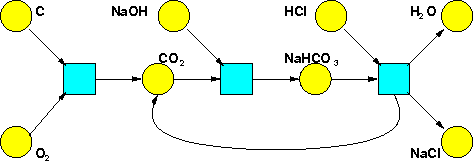
The states are in yellow, the transitions in blue. A labelling of our Petri net is a way of putting some number of things in each state. We can draw these things as little black dots:
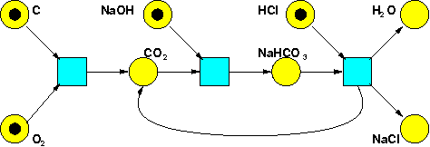
In this example there are only 0 or 1 things in each state: we've got one atom of carbon, one molecule of oxygen, one molecule of sodium hydroxide, one molecule of hydrochloric acid, and nothing else. But in general, we can have any natural number of things in each state.
In a stochastic Petri net, the transitions occur randomly as time passes. For example, as time passes we could see a sequence of transitions like this:


Each time a transition occurs, the number of things in each state changes in an obvious way.
In a stochastic Petri net, each transition has a rate constant, a nonnegative real number. Roughly speaking, this determines the probability of that transition.
A bit more precisely: suppose we have a Petri net that is labelled in some way at some moment. Then the probability that a given transition occurs in a short time $\Delta t$ is approximately:
• the rate constant for that transition, times
• the time $\Delta t$, times
• the number of ways the transition can occur.
More precisely still: this formula is correct up to terms of order $(\Delta t)^2$. So, taking the limit as $\Delta t \to 0$, we get a differential equation describing precisely how the probability of the Petri net having a given labelling changes with time! And this is the master equation.
Now, you might be impatient to actually see the master equation, but that would be rash. The true master doesn't need to see the master equation. It sounds like a Zen proverb, but it's true. The raw beginner in mathematics wants to see the solutions of an equation. The more advanced student is content to prove that the solution exists. But the master is content to prove that the equation exists.
A bit more seriously: what matters is understanding the rules that inevitably lead to some equation: actually writing it down is then straightforward.
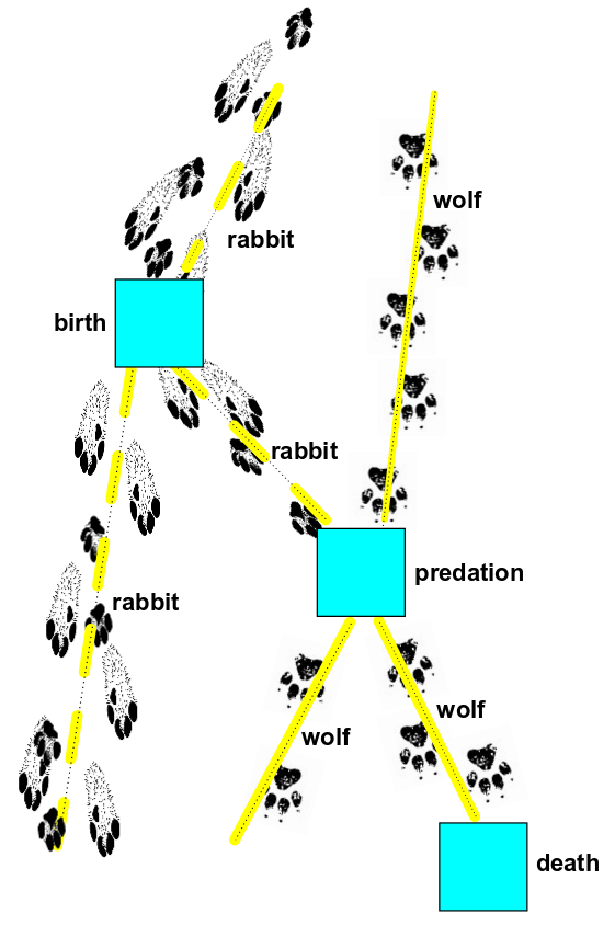
And you see, there's something I haven't explained yet: "the number of ways the transition can occur". This involves a bit of counting. Consider, for example, this Petri net:
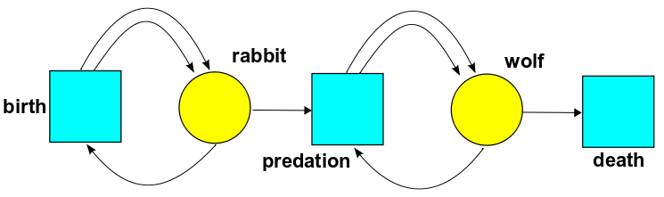
Suppose there are 10 rabbits and 5 wolves.
• How many ways can the birth transition occur? Since birth takes one rabbit as input, it can occur in 10 ways.
• How many ways can predation occur? Since predation takes one rabbit and one wolf as inputs, it can occur in 10 × 5 = 50 ways.
• How many ways can death occur? Since death takes one wolf as input, it can occur in 5 ways.
Or consider this one:
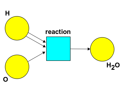
Suppose there are 10 hydrogen atoms and 5 oxygen atoms. How many ways can they form a water molecule? There are 10 ways to pick the first hydrogen, 9 ways to pick the second hydrogen, and 5 ways to pick the oxygen. So, there are $$ 10 \times 9 \times 5 = 450 $$ ways.
Note that we're treating the hydrogen atoms as distinguishable, so there are $10 \times 9$ ways to pick them, not $\frac{10 \times 9}{2} = {10 \choose 2}$. In general, the number of ways to choose $M$ distinguishable things from a collection of $L$ is the falling power $$ L^{\underline{M}} = L \cdot (L - 1) \cdots (L - M + 1) $$ where there are $M$ factors in the product, but each is 1 less than the preceding one—hence the term 'falling'.
Okay, now I've given you all the raw ingredients to work out the master equation for any stochastic Petri net. The previous paragraph was a big fat hint. One more nudge and you're on your own:
Puzzle. Suppose we have a stochastic Petri net with $k$ states and one transition with rate constant $r$. Suppose the $i$th state appears $m_i$ times as the input of this transition and $n_i$ times as the output. A labelling of this stochastic Petri net is a $k$-tuple of natural numbers $\ell = (\ell_1, \dots, \ell_k)$ saying how many things are in each state. Let $\psi_\ell(t)$ be the probability that the labelling is $\ell$ at time $t$. Then the master equation looks like this: $$ \frac{d}{d t} \psi_{\ell'}(t) = \sum_{\ell} H_{\ell' \ell} \psi_{\ell}(t) $$ for some matrix of real numbers $H_{\ell' \ell}.$ What is this matrix?
You can write down a formula for this matrix using what I've told you. And then, if you have a stochastic Petri net with more transitions, you can just compute the matrix for each transition using this formula, and add them all up.
There's a straightforward way to solve this puzzle, but I want to get the solution by a strange route: I want to guess the master equation using ideas from quantum field theory!
Some rabbits and wolves come in on top. They undergo some transitions as time passes, and go out on the bottom. The vertical coordinate is time, while the horizontal coordinate doesn't really mean anything: it just makes the diagram easier to draw.
If we ignore all the artistry that makes it cute, this Feynman diagram is just a graph with states as edges and transitions as vertices. Each transition occurs at a specific time.
We can use these Feynman diagrams to compute the probability that if we start it off with some labelling at time $t_1$, our stochastic Petri net will wind up with some other labelling at time $t_2$. To do this, we just take a sum over Feynman diagrams that start and end with the given labellings. For each Feynman diagram, we integrate over all possible times at which the transitions occur. And what do we integrate? Just the product of the rate constants for those transitions!
That was a bit of a mouthful, and it doesn't really matter if you followed it in detail. What matters is that it sounds a lot like stuff you learn when you study quantum field theory!
That's one clue that something cool is going on here. Another is the master equation itself: $$ \frac{d}{d t} \psi_{\ell'}(t) = \sum_{\ell} H_{\ell' \ell} \psi_{\ell}(t) $$ This looks a lot like Schrödinger's equation, the basic equation describing how a quantum system changes with the passage of time.
We can make it look even more like Schrödinger's equation if we create a vector space with the labellings $\ell$ as a basis. The numbers $\psi_\ell(t)$ will be the components of some vector $\psi(t)$ in this vector space. The numbers $H_{\ell' \ell}$ will be the matrix entries of some operator $H$ on that vector space. And the master equation becomes: $$ \frac{d}{d t} \psi(t) = H \psi(t) $$ Compare Schrödinger's equation: $$ i \frac{d}{d t} \psi(t) = H \psi(t) $$ The only visible difference is that factor of $i$!
But of course this is linked to another big difference: in the master equation $\psi$ describes probabilities, so it's a vector in a real vector space. In quantum theory $\psi$ describes probability amplitudes, so it's a vector in a complex Hilbert space.
Apart from this huge difference, everything is a lot like quantum field theory. In particular, our vector space is a lot like the Fock space one sees in quantum field theory. Suppose we have a quantum particle that can be in $k$ different states. Then its Fock space is the Hilbert space we use to describe an arbitrary collection of such particles. It has an orthonormal basis denoted $$ | \ell_1 \cdots \ell_k \rangle $$ where $\ell_1, \dots, \ell_k$ are natural numbers saying how many particles there are in each state. So, any vector in Fock space looks like this: $$ \psi = \sum_{\ell_1, \dots, \ell_k} \; \psi_{\ell_1 , \dots, \ell_k} \, | \ell_1 \cdots \ell_k \rangle $$ But if write the whole list $\ell_1, \dots, \ell_k$ simply as $\ell$, this becomes $$ \psi = \sum_{\ell} \psi_{\ell} | \ell \rangle $$ This is almost like what we've been doing with Petri nets!—except I hadn't gotten around to giving names to the basis vectors.
In quantum field theory class, I learned lots of interesting operators on Fock space: annihilation and creation operators, number operators, and so on. So, when I bumped into this master equation $$ \frac{d}{d t} \psi(t) = H \psi(t) $$ it seemed natural to take the operator $H$ and write it in terms of these. There was an obvious first guess, which didn't quite work... but thinking a bit harder eventually led to the right answer. Later, it turned out people had already thought about similar things. So, I want to explain this.
When I first started working on this stuff, I was focused on the difference between collections of indistinguishable things, like bosons or fermions, and collections of distinguishable things, like rabbits or wolves. But with the benefit of hindsight, it's even more important to think about the difference between quantum theory, which is all about probability amplitudes, and the game we're playing now, which is all about probabilities. So, next time I'll explain how we need to modify quantum theory so that it's about probabilities. This will make it easier to guess a nice formula for $H$.
You can also read comments on Azimuth, and make your own comments or ask questions there!
Here is the answer to the puzzle:
Puzzle. Suppose we have a stochastic Petri net with $k$ states and just one transition, whose rate constant is $r$. Suppose the $i$th state appears $m_i$ times as the input of this transition and $n_i$ times as the output. A labelling of this stochastic Petri net is a $k$-tuple of natural numbers $\ell = (\ell_1, \dots, \ell_k)$ saying how many things are in each state. Let $\psi_\ell(t)$ be the probability that the labelling is $\ell$ at time $t$. Then the master equation looks like this: $$\frac{d}{d t} \psi_{\ell'}(t) = \sum_{\ell} H_{\ell' \ell} \psi_{\ell}(t)$$ for some matrix of real numbers $ H_{\ell' \ell}$. What is this matrix?
Answer. To compute $H_{\ell' \ell}$ it's enough to start the Petri net in a definite labelling $\ell$ and see how fast the probability of being in some labelling $\ell'$ changes. In other words, if at some time $ t$ we have $$ \psi_{\ell}(t) = 1$$ then $$ \frac{d}{dt} \psi_{\ell'}(t) = H_{\ell' \ell}$$ at this time.
Now, suppose we have a Petri net that is labelled in some way at some moment. Then I said the probability that the transition occurs in a short time $ \Delta t$ is approximately:
• the rate constant $ r$, times
• the time $ \Delta t$, times
• the number of ways the transition can occur, which is the product of falling powers $ \ell_1^{\underline{m_1}} \cdots \ell_k^{\underline{m_k}}$. Let's call this product $ \ell^{\underline{m}}$ for short.
Multiplying these 3 things we get
$$ r \ell^{\underline{m}} \Delta t$$ So, the rate at which the transition occurs is just: $$ r \ell^{\underline{m}}$$ And when the transition occurs, it eats up $m_i$ things in the ith state, and produces $ n_i$ things in that state. So, it carries our system from the original labelling $ \ell$ to the new labelling $$ \ell' = \ell + n - m$$ So, in this case we have $$ \frac{d}{dt} \psi_{\ell'}(t) = r \ell^{\underline{m}}$$ and thus $$ H_{\ell' \ell} = r \ell^{\underline{m}}$$ However, that's not all: there's another case to consider! Since the probability of the Petri net being in this new labelling $ \ell'$ is going up, the probability of it staying in the original labelling $ \ell$ must be going down by the same amount. So we must also have $$ H_{\ell \ell} = - r \ell^{\underline{m}}$$ We can combine both cases into one formula like this: $$ H_{\ell' \ell} = r \ell^{\underline{m}} \left(\delta_{\ell', \ell + n - m} - \delta_{\ell', \ell}\right)$$ Here the first term tells us how fast the probability of being in the new labelling is going up. The second term tells us how fast the probability of staying in the original labelling is going down.
Note: each column in the matrix $ H_{\ell' \ell}$ sums to zero, and all the off-diagonal entries are nonnegative. That's good: next time we'll that this matrix must be 'infinitesimal stochastic', meaning precisely that it has these properties!
|
|
|
|