

|
|
|
|
You'll need to know a bit of math: calculus, a tiny bit probability theory, and linear operators on vector spaces. You don't need to know quantum theory, though you'll have more fun if you do. What we're doing here is very similar, but also strangely different—for reasons I explained last time.
$$ \Psi = \sum_{n = 0}^\infty \psi_n z^n $$
The variable $z$ doesn't mean anything in particular, and we don't care if the power series converges. See, in math 'formal' means "it's only symbols on the page, just follow the rules". It's like if someone says a party is 'formal', so need to wear a white tie: you're not supposed to ask what the tie means.
However, there's a good reason for this trick. We can define two operators on formal power series, called the annihilation operator:
$$ a \Psi = \frac{d}{d z} \Psi $$
and the creation operator:
$$ a^\dagger \Psi = z \Psi $$
They're just differentiation and multiplication by $z$, respectively. So, for example, suppose we start out being 100% sure we have $n$ rabbits for some particular number $n$. Then $\psi_n = 1$, while all the other probabilities are 0, so:
$$ \Psi = z^n $$
If we then apply the creation operator, we obtain
$$ a^\dagger \Psi = z^{n+1} $$
Voilà! One more rabbit!

The annihilation operator is more subtle. If we start out with $n$ rabbits:
$$ \Psi = z^n $$
and then apply the annihilation operator, we obtain
$$ a \Psi = n z^{n-1} $$
What does this mean? The $z^{n-1}$ means we have one fewer rabbit than before. But what about the factor of $n$? It means there were $n$ different ways we could pick a rabbit and make it disappear! This should seem a bit mysterious, for various reasons... but we'll see how it works soon enough.
The creation and annihilation operators don't commute: $$ (a a^\dagger - a^\dagger a) \Psi = \frac{d}{d z} (z \Psi) - z \frac{d}{d z} \Psi = \Psi $$ so for short we say: $$ a a^\dagger - a^\dagger a = 1 $$ or even shorter: $$ [a, a^\dagger] = 1 $$ where the commutator of two operators is $ [S,T] = S T - T S $.
The noncommutativity of operators is often claimed to be a special feature of quantum physics, and the creation and annihilation operators are fundamental to understanding the quantum harmonic oscillator. There, instead of rabbits, we're studying quanta of energy, which are peculiarly abstract entities obeying rather counterintuitive laws. So, it's cool that the same math applies to purely classical entities, like rabbits!
In particular, the equation $[a, a^\dagger] = 1$ just says that there's one more way to put a rabbit in a cage of rabbits, and then take one out, than to take one out and then put one in.
But how do we actually use this setup? We want to describe how the probabilities $\psi_n$ change with time, so we write
$$ \Psi(t) = \sum_{n = 0}^\infty \psi_n(t) z^n $$
Then, we write down an equation describing the rate of change of $\Psi$:
$$ \frac{d}{d t} \Psi(t) = H \Psi(t) $$
Here $H$ is an operator called the Hamiltonian, and the equation is called the master equation. The details of the Hamiltonian depend on our problem! But we can often write it down using creation and annihilation operators. Let's do some examples, and then I'll tell you the general rule.
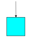
So, suppose an inexhaustible supply of rabbits are randomly roaming around a huge field, and each time a rabbit enters a certain area, we catch it and add it to our population of caged rabbits. Suppose that on average we catch one rabbit per unit time. Suppose the chance of catching a rabbit during any interval of time is independent of what happens before or afterwards. What is the Hamiltonian describing the probability distribution of caged rabbits, as a function of time?
There's an obvious dumb guess: the creation operator! However, we saw last time that this doesn't work, and we saw how to fix it. The right answer is $$H = a^\dagger - 1$$ To see why, suppose for example that at some time $t$ we have $n$ rabbits, so: $$\Psi(t) = z^n$$ Then the master equation says that at this moment, $$ \frac{d}{d t} \Psi(t) = (a^\dagger - 1) \Psi(t) = z^{n+1} - z^n$$ Since $\Psi = \sum_{n = 0}^\infty \psi_n(t) z^n$, this implies that the coefficients of our formal power series are changing like this: $$\frac{d}{d t} \psi_{n+1}(t) = 1 $$ $$\frac{d}{d t} \psi_{n}(t) = -1$$ while all the rest have zero derivative at this moment. And that's exactly right! See, $\psi_{n+1}(t)$ is the probability of having one more rabbit, and this is going up at rate 1. Meanwhile, $\psi_n(t)$ is the probability of having $n$ rabbits, and this is going down at the same rate.
Puzzle 1. Show that with this Hamiltonian and any initial conditions, the master equation predicts that the expected number of rabbits grows linearly.
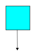
Suppose a mean nasty guy had a population of rabbits in a cage and didn't feed them at all. Suppose that each rabbit has a unit probability of dying per unit time. And as always, suppose the probability of this happening in any interval of time is independent of what happens before or after that time.
What is the Hamiltonian? Again there's a dumb guess: the annihilation operator! And again this guess is wrong, but it's not far off. As before, the right answer includes a 'correction term': $$ H = a - N $$ This time the correction term is famous in its own right. It's called the number operator: $$N = a^\dagger a $$ The reason is that if we start with $n$ rabbits, and apply this operator, it amounts to multiplication by $n$: $$ N z^n = z \frac{d}{d z} z^n = n z^n $$ Let's see why this guess is right. Again, suppose that at some particular time $t$ we have $n$ rabbits, so $$\Psi(t) = z^n$$ Then the master equation says that at this time $$ \frac{d}{d t} \Psi(t) = (a - N) \Psi(t) = n z^{n-1} - n z^n$$ So, our probabilities are changing like this: $$\frac{d}{d t} \psi_{n-1}(t) = n $$ $$\frac{d}{d t} \psi_n(t) = -n$$ while the rest have zero derivative. And this is good! We're starting with $n$ rabbits, and each has a unit probability per unit time of dying. So, the chance of having one less should be going up at rate $n$. And the chance of having the same number we started with should be going down at the same rate.
Puzzle 2. Show that with this Hamiltonian and any initial conditions, the master equation predicts that the expected number of rabbits decays exponentially.
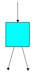
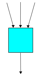
As you can see from the cryptic picture above, this 'duplication' process takes one rabbit as input and has two rabbits as output. So, if you've been paying attention, you should be ready with a dumb guess for the Hamiltonian: $a^\dagger a^\dagger a$. This operator annihilates one rabbit and then creates two!
But you should also suspect that this dumb guess will need a 'correction term'. And you're right! As always, the correction terms makes the probability of things staying the same go down at exactly the rate that the probability of things changing goes up.
You should guess the correction term... but I'll just tell you: $$ H = a^\dagger a^\dagger a - N $$ We can check this in the usual way, by seeing what it does when we have $n$ rabbits: $$ H z^n = z^2 \frac{d}{d z} z^n - n z^n = n z^{n+1} - n z^n $$ That's good: since there are $n$ rabbits, the rate of rabbit duplication is $n$. This is the rate at which the probability of having one more rabbit goes up... and also the rate at which the probability of having $n$ rabbits goes down.
Puzzle 3. Show that with this Hamiltonian and any initial conditions, the master equation predicts that the expected number of rabbits grows exponentially.
(If you prefer unordered pairs of rabbits, just divide the Hamiltonian by 2. We should talk about this more, but not now.)
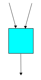
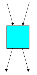
Now each triple of rabbits has a unit probability per unit time of getting into a fight with only one survivor! I don't know the technical term for a three-way fight, but perhaps it counts as a small 'brawl' or 'melee'. In fact the Wikipedia article for 'melee' shows three rabbits in suits of armor, fighting it out:

Now the Hamiltonian is: $$ H = a^\dagger a^3 - N(N-1)(N-2) $$ You can check that: $$ H z^n = n(n-1)(n-2) z^{n-2} - n(n-1)(n-2) z^n $$ and this is good, because $n(n-1)(n-2)$ is the number of ordered triples of rabbits. You can see how this number shows up from the math, too: $$ a^3 z^n = \frac{d^3}{d z^3} z^n = n(n-1)(n-2) z^{n-3} $$
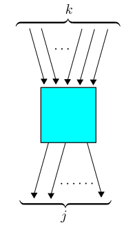
There's another nice little lesson here. Copying the calculation we just did, it's easy to see that: $$ {a^{\dagger}}^k a^k = N^{\underline{k}}$$ This is a cute formula for falling powers of the number operator in terms of annihilation and creation operators. It means that for the general transition we saw before:
Okay, that's it for now! We can, and will, generalize all this stuff to stochastic Petri nets where there are things of many different kinds—not just rabbits. And we'll see that the master equation we get matches the answer to the puzzle in Part 4. That's pretty easy. But first, we'll have a guest post by Jacob Biamonte, who will explain a more realistic example from population biology.
You can also read comments on Azimuth, and make your own comments or ask questions there!
Here are the answers to the puzzles:
Puzzle 1. Show that with the Hamiltonian $$H = a^\dagger - 1$$ and any initial conditions, the master equation predicts that the expected number of rabbits grows linearly.
Answer. Here is one answer, thanks to David Corfield on Azimuth. If at some time $t$ we have $n$ rabbits, so that $\Psi(t) = z^n$, we have seen that the probability of having any number of rabbits changes as follows: $$\frac{d}{d t} \psi_{n+1}(t) = 1, \qquad \frac{d}{d t} \psi_{n}(t) = -1, \qquad \frac{d}{d t} \psi_m(t) = 0 \mathrm{\; \; otherwise} $$ Thus the rate of increase of the expected number of rabbits is $(n + 1) - n = 1$. But any probability distribution is a linear combination of these basis vector $z^n$, so the rate of increase of the expected number of rabbits is always $$\sum_n \psi_{n}(t) = 1$$ so the expected number grows linearly.
Here is a second solution, using some more machinery. This machinery is overkill here, but it will be useful for solving the next two puzzles and also many other problems.
In the general formalism described last time, I used $\int \psi$ to mean the integral of a function over some measure space, so that probability distributions are the functions obeying $$\int \psi = 1$$ and $$\psi \ge 0$$ In the examples today this integral is really a sum over $n = 0,1,2, \dots$, and it might be confusing to use integral notation since we're using derivatives for a completely different purpose. So let me define a sum notation as follows: $$\sum \Psi = \sum_{n = 0}^\infty \psi_n $$ This may be annoying, since after all we really have $$\Psi|_{z = 1} = \sum_{n = 0}^\infty \psi_n $$ but please humor me.
To work with this sum notation, two rules are very handy.
Rule 1: For any formal power series $\Phi$, \[ \sum a^\dagger \Phi = \sum \Phi \] I mentioned this last time: it's part of the creation operator being a stochastic operator. It's easy to check: $$ \sum a^\dagger \Phi = z \Phi|_{z = 1} = \Phi|_{z=1} = \sum \Phi $$
Rule 2: For any formal power series $\Phi$, $$ \sum a \Phi = \sum N \Phi $$ Again this is easy to check: $$\sum N \Phi = \sum a^\dagger a \Phi = \sum a \Phi $$ These rules can be used together with the commutation relation $$ [a , a^\dagger] = 1 $$ and its consequences $$ [a, N] = a, \qquad [a^\dagger, N] = - a^\dagger $$ to do many interesting things.
Let's see how! Suppose we have some observable $O$ that we can write as an operator on formal power series: for example, the number operator, or any power of that. The expected value of this observable in the probability distribution $\Psi$ is $$\sum O \Psi $$ So, if we're trying to work out the time derivative of the expected value of $O$, we can start by using the master equation: $$ \frac{d}{dt} \sum O \Psi(t) = \sum O \frac{d}{dt} \Psi(t) = \sum O H \Psi(t) $$ Then we can write $O$ and $H$ using annihilation and creation operators and use our rules.
For example, in the puzzle at hand, we have $$H = a^\dagger - 1 $$ and the observable we're interested in is the number of rabbits $$O = N$$ so we want to compute $$\sum O H \Psi(t) = \sum N(a^\dagger - 1) \Psi(t) $$ There are many ways to use our rules to evaluate this. For example, Rule 1 implies that $$\sum N(a^\dagger - 1) \Psi(t) = \sum a(a^\dagger - 1)\Psi(t) $$ but the commutation relations say $a a^\dagger = a^\dagger a + 1 = N+1$, so $$ \sum a(a^\dagger - 1)\Psi(t) = \sum (N + 1 - a) \Psi(t) $$ and using Rule 1 again we see this equals $$ \sum \Psi(t) = 1 $$ Thus we have $$ \frac{d}{dt} \sum N \Psi(t) = 1 $$ It follows that the expected number of rabbits grows linearly: $$ \sum N \Psi(t) = t + c $$
Puzzle 2. Show that with the Hamiltonian $$ H = a - N $$ and any initial conditions, the master equation predicts that the expected number of rabbits decays exponentially.
Answer. We use the machinery developed in our answer to Puzzle 1. We want to compute the time derivative of the expected number of rabbits: $$ \frac{d}{dt} \sum N \Psi = \sum N H \Psi = \sum N (a - N) \Psi $$ The commutation relation $[a, N] = a$ implies that $Na = aN - a$. So: $$ \sum N(a-N) \Psi = \sum (a N - N - N^2) \Psi$$ but now Rule 2 says: $$ \sum (a N - N - N^2)\Psi = \sum (N^2 - N - N^2) \Psi = - \sum N \Psi $$ so we see $$\frac{d}{dt} \sum N \Psi = - \sum N \Psi$$ It follows that the expected number of rabbits decreases exponentially: $$ \sum N \Psi(t) = c e^{-t} $$
Puzzle 3. Show that with the Hamiltonian $$H = {a^\dagger}^2 a - N $$ and any initial conditions, the master equation predicts that the expected number of rabbits grows exponentially.
Answer. We use the same technique to compute $$ \frac{d}{dt} \sum N \Psi(t) = \sum N H \Psi(t) = \sum (N {a^\dagger}^2 a - N) \Psi(t) $$ First use the commutation relations to note: $$ N({a^\dagger}^2 a - N) = N a^\dagger N - N^2 = a^\dagger (N+1) N - N^2$$ Then: $$ \sum (a^\dagger (N+1) N - N^2) \Psi(t) = \sum ((N+1)N -N^2) \Psi(t) = \sum N \Psi(t) $$ So, we have $$ \frac{d}{dt} \sum N \Psi(t) = \sum N \Psi(t) $$ It follows that the expected number of rabbits grows exponentially: $$ \sum N \Psi(t) = c e^t $$
|
|
|
|