

|
|
|
|
This month, before he goes to Oxford to begin a master's program in Mathematics and the Foundations of Computer Science, Brendan Fong is visiting the Centre for Quantum Technologies and working with me on stochastic Petri nets. He's proved two interesting results, which he wants to explain.
To understand what he's done, you need to know how to get the rate equation and the master equation from a stochastic Petri net. We've almost seen how. But it's been a long time since the last article in this series, so today I'll start with some review. And at the end, just for fun, I'll say a bit more about how Feynman diagrams show up in this theory.
Since I'm an experienced teacher, I'll assume you've forgotten everything I ever said.
(This has some advantages. I can change some of my earlier terminology—improve it a bit here and there—and you won't even notice.)
Definition. A Petri net consists of a set $S$ of species and a set $T$ of transitions, together with a function $$ i : S \times T \to \mathbb{N} $$ saying how many things of each species appear in the input for each transition, and a function $$ o: S \times T \to \mathbb{N}$$ saying how many things of each species appear in the output.
We can draw pictures of Petri nets. For example, here's a Petri net with two species and three transitions:
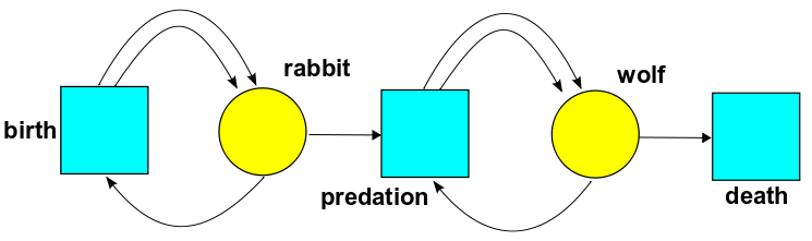
It should be clear that the transition 'predation' has one wolf and one rabbit as input, and two wolves as output.
A 'stochastic' Petri net goes further: it also says the rate at which each transition occurs.
Definition. A stochastic Petri net is a Petri net together with a function $$ r: T \to (0,\infty) $$ giving a rate constant for each transition.
Starting from any stochastic Petri net, we can get two things. First:
The master equation is stochastic: it describes how probabilities change with time. The rate equation is deterministic.
The master equation is more fundamental. It's like the equations of quantum electrodynamics, which describe the amplitudes for creating and annihilating individual photons. The rate equation is less fundamental. It's like the classical Maxwell equations, which describe changes in the electromagnetic field in a deterministic way. The classical Maxwell equations are an approximation to quantum electrodynamics. This approximation gets good in the limit where there are lots of photons all piling on top of each other to form nice waves.
Similarly, the rate equation can be derived from the master equation in the limit where the number of things of each species become large, and the fluctuations in these numbers become negligible.
But I won't do this derivation today! Nor will I probe more deeply into the analogy with quantum field theory, even though that's my ultimate goal. Today I'm content to remind you what the master equation and rate equation are.
The rate equation is simpler, so let's do that first.
Suppose we have a stochastic Petri net with $k$ different species. Let $x_i$ be the number of things of the $i$th species. Then the rate equation looks like this:
$$ \frac{d x_i}{d t} = ??? $$
It's really a bunch of equations, one for each $1 \le i \le k$. But what is the right-hand side?
The right-hand side is a sum of terms, one for each transition in our Petri net. So, let's start by assuming our Petri net has just one transition.
Suppose the $i$th species appears as input to this transition $m_i$ times, and as output $n_i$ times. Then the rate equation is
$$ \frac{d x_i}{d t} = r (n_i - m_i) x_1^{m_1} \cdots x_k^{m_k} $$
where $r$ is the rate constant for this transition.
That's really all there is to it! But we can make it look nicer. Let's make up a vector
$$ x = (x_1, \dots , x_k) \in [0,\infty)^k $$
that says how many things there are of each species. Similarly let's make up an input vector
$$ m = (m_1, \dots, m_k) \in \mathbb{N}^k $$
and an output vector
$$ n = (n_1, \dots, n_k) \in \mathbb{N}^k $$
for our transition. To be cute, let's also define
$$ x^m = x_1^{m_1} \cdots x_k^{m_k} $$
Then we can write the rate equation for a single transition like this:
$$ \frac{d x}{d t} = r (n-m) x^m $$
Next let's do a general stochastic Petri net, with lots of transitions. Let's write $T$ for the set of transitions and $r(\tau)$ for the rate constant of the transition $\tau \in T$. Let $n(\tau)$ and $m(\tau)$ be the input and output vectors of the transition $\tau$. Then the rate equation is:
$$ \frac{d x}{d t} = \sum_{\tau \in T} r(\tau) \, (n(\tau) - m(\tau)) \, x^{m(\tau)} $$
For example, consider our rabbits and wolves:
Suppose
Let $x_1(t)$ be the number of rabbits and $x_2(t)$ the number of wolves at time $t$. Then the rate equation looks like this:
$$ \frac{d x_1}{d t} = \beta x_1 - \gamma x_1 x_2 $$
$$ \frac{d x_2}{d t} = \gamma x_1 x_2 - \delta x_2 $$
If you stare at this, and think about it, it should make perfect sense. If it doesn't, go back and read Part 2.
Now let's do something new. In Part 6 I explained how to write down the master equation for a stochastic Petri net with just one species. Now let's generalize that. Luckily, the ideas are exactly the same.
So, suppose we have a stochastic Petri net with $k$ different species. Let $\psi_{n_1, \dots, n_k}$ be the probability that we have $n_1$ things of the first species, $n_2$ of the second species, and so on. The master equation will say how all these probabilities change with time.
To keep the notation clean, let's introduce a vector
$$ n = (n_1, \dots, n_k) \in \mathbb{N}^k $$
and let
$$ \psi_n = \psi_{n_1, \dots, n_k} $$
Then, let's take all these probabilities and cook up a formal power series that has them as coefficients: as we've seen, this is a powerful trick. To do this, we'll bring in some variables $z_1, \dots, z_k$ and write
$$ z^n = z_1^{n_1} \cdots z_k^{n_k} $$
as a convenient abbreviation. Then any formal power series in these variables looks like this:
$$ \Psi = \sum_{n \in \mathbb{N}^k} \psi_n z^n $$
We call $\Psi$ a state if the probabilities sum to 1 as they should:
$$ \sum_n \psi_n = 1 $$
The simplest example of a state is a monomial:
$$ z^n = z_1^{n_1} \cdots z_k^{n_k} $$
This is a state where we are 100% sure that there are $n_1$ things of the first species, $n_2$ of the second species, and so on. We call such a state a pure state, since physicists use this term to describe a state where we know for sure exactly what's going on. Sometimes a general state, one that might not be pure, is called mixed.
The master equation says how a state evolves in time. It looks like this:
$$ \frac{d}{d t} \Psi(t) = H \Psi(t) $$
So, I just need to tell you what $H$ is!
It's called the Hamiltonian. It's a linear operator built from special operators that annihilate and create things of various species. Namely, for each state $1 \le i \le k$ we have a annihilation operator:
$$ a_i \Psi = \frac{d}{d z_i} \Psi $$
and a creation operator:
$$ a_i^\dagger \Psi = z_i \Psi $$
How do we build $H$ from these? Suppose we've got a stochastic Petri net whose set of transitions is $T$. As before, write $r(\tau)$ for the rate constant of the transition $\tau \in T$, and let $n(\tau)$ and $m(\tau)$ be the input and output vectors of this transition. Then:
$$ H = \sum_{\tau \in T} r(\tau) \, ({a^\dagger}^{n(\tau)} - {a^\dagger}^{m(\tau)}) \, a^{m(\tau)} $$
where as usual we've introduce some shorthand notations to keep from going insane. For example:
$$ a^{m(\tau)} = a_1^{m_1(\tau)} \cdots a_k^{m_k(\tau)} $$
and
$$ {a^\dagger}^{m(\tau)} = {a_1^\dagger }^{m_1(\tau)} \cdots {a_k^\dagger}^{m_k(\tau)} $$
Now, it's not surprising that each transition $\tau$ contributes a term to $H$. It's also not surprising that this term is proportional to the rate constant $r(\tau)$. The only tricky thing is the expression
$$ ({a^\dagger}^{n(\tau)} - {a^\dagger}^{m(\tau)})a^{m(\tau)} $$
How can we understand it? The basic idea is this. We've got two terms here. The first term:
$$ {a^\dagger}^{n(\tau)} a^{m(\tau)} $$
describes how $m_i(\tau)$ things of the $i$th species get annihilated, and $n_i(\tau)$ things of the $i$th species get created. Of course this happens thanks to our transition $\tau$. The second term:
$$ - {a^\dagger}^{m(\tau)} a^{m(\tau)} $$
is a bit harder to understand, but it says how the probability that nothing happens—that we remain in the same pure state—decreases as time passes. Again this happens due to our transition $\tau$.
In fact, the second term must take precisely the form it does to ensure 'conservation of total probability'. In other words: if the probabilities $\psi_n$ sum to 1 at time zero, we want these probabilities to still sum to 1 at any later time. And for this, we need that second term to be what it is! In Part 6 we saw this in the special case where there's only one species. The general case works the same way.
Let's look at an example. Consider our rabbits and wolves yet again:
and again suppose the rate constants for birth, predation and death are $\beta$, $\gamma$ and $\delta$, respectively. We have
$$ \Psi = \sum_n \psi_n z^n $$
where
$$ z^n = z_1^{n_1} z_2^{n_2} $$
and $\psi_n = \psi_{n_1, n_2}$ is the probability of having $n_1$ rabbits and $n_2$ wolves. These probabilities evolve according to the equation
$$ \frac{d}{d t} \Psi(t) = H \Psi(t) $$
where the Hamiltonian is
$$ H = \beta B + \gamma C + \delta D $$
and $B$, $C$ and $D$ are operators describing birth, predation and death, respectively. ($B$ stands for birth, $D$ stands for death... and you can call predation 'consumption' if you want something that starts with $C$. Besides, 'consumer' is a nice euphemism for 'predator'.) What are these operators? Just follow the rules I described:
$$ B = {a_1^\dagger}^2 a_1 - a_1^\dagger a_1$$
$$ C = {a_2^\dagger}^2 a_1 a_2 - a_1^\dagger a_2^\dagger a_1 a_2 $$
$$ D = a_2 - a_2^\dagger a_2 $$
In each case, the first term is easy to understand:
The second term is trickier, but I told you how it works.
How do we solve the master equation? If we don't worry about mathematical rigor too much, it's easy. The solution of
$$ \frac{d}{d t} \Psi(t) = H \Psi(t) $$
should be
$$ \Psi(t) = e^{t H} \Psi(0) $$
and we can hope that
$$ e^{t H} = 1 + t H + \frac{(t H)^2}{2!} + \cdots $$
so that
$$ \Psi(t) = \Psi(0) + t H \Psi(0) + \frac{t^2}{2!} H^2 \Psi(0) + \cdots $$
Of course there's always the question of whether this power series converges. In many contexts it doesn't, but that's not necessarily a disaster: the series can still be asymptotic to the right answer, or even better, Borel summable to the right answer.
But let's not worry about these subtleties yet! Let's just imagine our rabbits and wolves, with Hamiltonian
$$ H = \beta B + \gamma C + \delta D $$
Now, imagine working out
$$ \Psi(t) = \Psi(0) + t H \Psi(0) + \frac{t^2}{2!} H^2 \Psi(0) + \frac{t^3}{3!} H^3 \Psi(0) + \cdots $$
We'll get lots of terms involving products of $B$, $C$ and $D$ hitting our original state $\Psi(0)$. And we can draw these as diagrams! For example, suppose we start with one rabbit and one wolf. Then
$$ \Psi(0) = z_1 z_2 $$
And suppose we want to compute
$$ H^3 \Psi(0) = (\beta B + \gamma C + \delta D)^3 \Psi(0) $$
as part of the task of computing $\Psi(t)$. Then we'll get lots of terms: 27, in fact, though many will turn out to be zero. Let's take one of these terms, for example the one proportional to:
$$ D C B \Psi(0) $$
We can draw this as a sum of Feynman diagrams, including this:
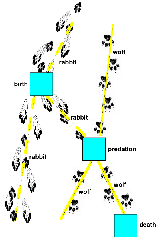
In this diagram, we start with one rabbit and one wolf at top. As we read the diagram from top to bottom, first a rabbit is born ($B$), then predation occur ($C$), and finally a wolf dies ($D$). The end result is again a rabbit and a wolf.
This is just one of four Feynman diagrams we should draw in our sum for $D C B \Psi(0)$, since either of the two rabbits could have been eaten, and either wolf could have died. So, the end result of computing
$$ H^3 \Psi(0) $$
will involve a lot of Feynman diagrams... and of course computing
$$ \Psi(t) = \Psi(0) + t H \Psi(0) + \frac{t^2}{2!} H^2 \Psi(0) + \frac{t^3}{3!} H^3 \Psi(0) + \cdots $$
will involve even more, even if we get tired and give up after the first few terms. So, this Feynman diagram business may seem quite tedious... and it may not be obvious how it helps.
But it does, sometimes!
Now is not the time for me to describe 'practical' benefits of Feynman diagrams. Instead, I'll just point out one conceptual benefit. We started with what seemed like a purely computational chore, namely computing
$$ \Psi(t) = \Psi(0) + t H \Psi(0) + \frac{t^2}{2!} H^2 \Psi(0) + \cdots $$
But then we saw—at least roughly—how this series has a clear meaning! It can be written as a sum over diagrams, each of which represents a possible history of rabbits and wolves. So, it's what physicists call a 'sum over histories'.
Feynman invented the idea of a sum over histories in the context of quantum field theory. At the time this idea seemed quite mind-blowing, for various reasons. First, it involved elementary particles instead of everyday things like rabbits and wolves. Second, it involved complex 'amplitudes' instead of real probabilities. Third, it actually involved integrals instead of sums. And fourth, a lot of these integrals diverged, giving infinite answers that needed to be 'cured' somehow!
Now we're seeing a sum over histories in a more down-to-earth context without all these complications. A lot of the underlying math is analogous... but now there's nothing mind-blowing about it: it's quite easy to understand. So, we can use this analogy to demystify quantum field theory a bit. On the other hand, thanks to this analogy, all sorts of clever ideas invented by quantum field theorists will turn out to have applications to biology and chemistry! So it's a double win.
You can also read comments on Azimuth, and make your own comments or ask questions there!
|
|
|
|