

|
|
|
|
Last time we reviewed the rate equation and the master equation. Both of them describe processes where things of various kinds can react and turn into other things. But:
This should remind you of the difference between classical mechanics and quantum mechanics. But the master equation is not quantum, it's stochastic: it involves probabilities, but there's no uncertainty principle going on.
Still, a lot of the math is similar.
Now, given an equilibrium solution to the rate equation—one that doesn't change with time—we'll try to find a solution to the master equation with the same property. We won't always succeed—but we often can! The theorem saying how was proved here:
To emphasize the analogy to quantum mechanics, we'll translate their proof into the language of annihilation and creation operators. In particular, our equilibrium solution of the master equation is just like what people call a 'coherent state' in quantum mechanics.
So, if you know about quantum mechanics and coherent states, you should be happy. But if you don't, fear not!—we're not assuming you do.
To construct our equilibrium solution of the master equation, we need a special type of solution to our rate equation. We call this type a 'complex balanced solution'. This means that not only is the net rate of production of each species zero, but the net rate of production of each possible bunch of species is zero.
Before we make this more precise, let's remind ourselves of the basic setup.
We'll consider a stochastic Petri net with a finite set $ S$ of species and a finite set $ T$ of transitions. For convenience let's take $ S = \{1,\dots, k\}$, so our species are numbered from 1 to $ k$. Then each transition $ \tau$ has an input vector $ m(\tau) \in \mathbb{N}^k$ and output vector $ n(\tau) \in \mathbb{N}^k$. These say how many things of each species go in, and how many go out. Each transition also has rate constant $ r(\tau) \in (0,\infty)$, which says how rapidly it happens.
The rate equation concerns a vector $ x(t) \in [0,\infty)^k$ whose $ i$th component is the number of things of the $ i$th species at time $ t$. Note: we're assuming this number of things varies continuously and is known precisely! This should remind you of classical mechanics. So, we'll call $ x(t)$, or indeed any vector in $ [0,\infty)^k$, a classical state.
The rate equation says how the classical state $ x(t)$ changes with time:
$$ \displaystyle{ \frac{d x}{d t} = \sum_{\tau \in T} r(\tau)\, (n(\tau)-m(\tau)) \, x^{m(\tau)} } $$
You may wonder what $ x^{m(\tau)}$ means: after all, we're taking a vector to a vector power! It's just an abbreviation, which we've seen plenty of times before. If $ x \in \mathbb{R}^k$ is a list of numbers and $ m \in \mathbb{N}^k$ is a list of natural numbers, we define
$$ x^m = x_1^{m_1} \cdots x_k^{m_k} $$
We'll also use this notation when $ x$ is a list of operators.
The vectors $ m(\tau)$ and $ n(\tau)$ are examples of what chemists call complexes. A complex is a bunch of things of each species. For example, if the set $ S$ consists of three species, the complex $ (1,0,5)$ is a bunch consisting of one thing of the first species, none of the second species, and five of the third species.
For our Petri net, the set of complexes is the set $ \mathbb{N}^k$, and the complexes of particular interest are the input complex $ m(\tau)$ and the output complex $ n(\tau)$ of each transition $ \tau$.
We say a classical state $ c \in [0,\infty)^k$ is complex balanced if for all complexes $ \kappa \in \mathbb{N}^k$ we have
$$ \displaystyle{ \sum_{\{\tau : m(\tau) = \kappa\}} r(\tau) c^{m(\tau)} =\sum_{\{\tau : n(\tau) = \kappa\}} r(\tau) c^{m(\tau)} } $$
The left hand side of this equation, which sums over the transitions with input complex $ \kappa$, gives the rate of consumption of the complex $ \kappa .$ The right hand side, which sums over the transitions with output complex $ \kappa$, gives the rate of production of $ \kappa .$ So, this equation requires that the net rate of production of the complex $ \kappa$ is zero in the classical state $ c .$
Puzzle. Show that if a classical state $ c$ is complex balanced, and we set $ x(t) = c$ for all $ t,$ then $ x(t)$ is a solution of the rate equation.
Since $ x(t)$ doesn't change with time here, we call it an equilibrium solution of the rate equation. Since $ x(t) = c$ is complex balanced, we call it complex balanced equilibrium solution.
We've seen that any complex balanced classical state gives an equilibrium solution of the rate equation. The Anderson–Craciun–Kurtz theorem says that it also gives an equilibrium solution of the master equation. The master equation concerns a formal power series
$$ \displaystyle{ \Psi(t) = \sum_{n \in \mathbb{N}^k} \psi_n(t) z^n } $$
where
$$ z^n = z_1^{n_1} \cdots z_k^{n_k} $$
and
$$ \psi_n(t) = \psi_{n_1, \dots,n_k}(t) $$
is the probability that at time $ t$ we have $ n_1$ things of the first species, $ n_2$ of the second species, and so on.
Note: now we're assuming this number of things varies discretely and is known only probabilistically! So, we'll call $ \Psi(t)$, or indeed any formal power series where the coefficients are probabilities summing to 1, a stochastic state. Earlier we just called it a 'state', but that would get confusing now: we've got classical states and stochastic states, and we're trying to relate them.
The master equation says how the stochastic state $ \Psi(t)$ changes with time:
$$ \displaystyle{ \frac{d}{d t} \Psi(t) = H \Psi(t) } $$
where the Hamiltonian $ H$ is:
$$ \displaystyle{ H = \sum_{\tau \in T} r(\tau) \left({a^\dagger}^{n(\tau)} - {a^\dagger}^{m(\tau)} \right) a^{m(\tau)} } $$
The notation here is designed to neatly summarize some big products of annihilation and creation operators. For any vector $ n \in \mathbb{N}^k$, we have
$$ a^n = a_1^{n_1} \cdots a_k^{n_k} $$
and
$$ \displaystyle{ {a^\dagger}^n = {a_1^\dagger }^{n_1} \cdots {a_k^\dagger}^{n_k} } $$
Now suppose $ c \in [0,\infty)^k$ is a complex balanced equilibrium solution of the rate equation. We want to get an equilibrium solution of the master equation. How do we do it?
For any $ c \in [0,\infty)^k$ there is a stochastic state called a coherent state, defined by
$$ \displaystyle{ \Psi_c = \frac{e^{c z}}{e^c} } $$
Here we are using some very terse abbreviations. Namely, we are defining
$$ e^{c} = e^{c_1} \cdots e^{c_k} $$
and
$$ e^{c z} = e^{c_1 z_1} \cdots e^{c_k z_k} $$
Equivalently,$$ \displaystyle{ e^{c z} = \sum_{n \in \mathbb{N}^k} \frac{c^n}{n!}z^n } $$
where $c^n$ and $z^n$ are defined as products in our usual way, and
$$ n! = n_1! \, \cdots \, n_k! $$
Either way, if you unravel the abbrevations, here's what you get:
$$ \displaystyle{ \Psi_c = e^{-(c_1 + \cdots + c_k)} \, \sum_{n \in \mathbb{N}^k} \frac{c_1^{n_1} \cdots c_k^{n_k}} {n_1! \, \cdots \, n_k! } \, z_1^{n_1} \cdots z_k^{n_k} } $$
Maybe now you see why we like the abbreviations.
The name 'coherent state' comes from quantum mechanics. In quantum mechanics, we think of a coherent state $ \Psi_c$ as the 'quantum state' that best approximates the classical state $ c$. But we're not doing quantum mechanics now, we're doing probability theory. $ \Psi_c$ isn't a 'quantum state', it's a stochastic state.
In probability theory, people like Poisson distributions. In the state $ \Psi_c$, the probability of having $ n_i$ things of the $ i$th species is equal to
$$ \displaystyle{ e^{-c_i} \, \frac{c_i^{n_i}}{n_i!} } $$
This is precisely the definition of a Poisson distribution with mean equal to $ c_i$. We can multiply a bunch of factors like this, one for each species, to get
$$ \displaystyle{ e^{-c} \, \frac{c^n}{n!} } $$
This is the probability of having $ n_1$ things of the first species, $ n_2$ things of the second, and so on, in the state $ \Psi_c$. So, the state $ \Psi_c$ is a product of independent Poisson distributions. In particular, knowing how many things there are of one species says nothing all about how many things there are of any other species!
It is remarkable that such a simple state can give an equilibrium solution of the master equation, even for very complicated stochastic Petri nets. But it's true—at least if $ c$ is complex balanced.
Now we're ready to state and prove the big result:
Theorem (Anderson–Craciun–Kurtz). Suppose $ c \in [0,\infty)^k$ is a complex balanced equilibrium solution of the rate equation. Then $ H \Psi_c = 0$.
It follows that $ \Psi_c$ is an equilibrium solution of the master equation. In other words, if we take $ \Psi(t) = \Psi_c$ for all times $ t$, the master equation holds:
$$ \displaystyle{ \frac{d}{d t} \Psi(t) = H \Psi(t) } $$
since both sides are zero.
Proof. To prove the Anderson–Craciun–Kurtz theorem, we just need to show that $ H \Psi_c = 0$. Since $ \Psi_c$ is a constant times $ e^{c z}$, it suffices to show $ H e^{c z} = 0$. Remember that
$$ \displaystyle{ H e^{c z} = \sum_{\tau \in T} r(\tau) \left( {a^\dagger}^{n(\tau)} -{a^\dagger}^{m(\tau)} \right) \, a^{m(\tau)} \, e^{c z} } $$
Since the annihilation operator $ a_i$ is given by differentiation with respect to $ z_i$, while the creation operator $ a^\dagger_i$ is just multiplying by $ z_i$, we have:
$$ \displaystyle{ H e^{c z} = \sum_{\tau \in T} r(\tau) \, c^{m(\tau)} \left( z^{n(\tau)} - z^{m(\tau)} \right) e^{c z} } $$
Expanding out $ e^{c z}$ we get:
$$ \displaystyle{ H e^{c z} = \sum_{i \in \mathbb{N}^k} \sum_{\tau \in T} r(\tau)c^{m(\tau)}\left(z^{n(\tau)}\frac{c^i}{i!}z^i - z^{m(\tau)}\frac{c^i}{i!}z^i\right) } $$
Shifting indices and defining negative powers to be zero:
$$ \displaystyle{ H e^{c z} = \sum_{i \in \mathbb{N}^k} \sum_{\tau \in T} r(\tau)c^{m(\tau)}\left(\frac{c^{i-n(\tau)}}{(i-n(\tau))!}z^i - \frac{c^{i-m(\tau)}}{(i-m(\tau))!}z^i\right) } $$
So, to show $ H e^{c z} = 0$, we need to show this:
$$ \displaystyle{ \sum_{i \in \mathbb{N}^k} \sum_{\tau \in T} r(\tau)c^{m(\tau)}\frac{c^{i-n(\tau)}}{(i-n(\tau))!} \, z^i =\sum_{i \in \mathbb{N}^k} \sum_{\tau \in T} r(\tau)c^{m(\tau)}\frac{c^{i-m(\tau)}}{(i-m(\tau))!} \,z^i } $$
We do this by splitting the sum over $ T$ according to output and then input complexes, making use of the complex balanced condition:
$$ \begin{array}{ccl} \displaystyle{ \sum_{i \in \mathbb{N}^k} \sum_{\kappa \in \mathbb{N}^k} \sum_{\{\tau : n(\tau)=\kappa\}} r(\tau)c^{m(\tau)}\frac{c^{i-n(\tau)}}{(i-n(\tau))!} \, z^i } &=& \sum_{i \in \mathbb{N}^k} \sum_{\kappa \in \mathbb{N}^k} \frac{c^{i-\kappa}}{(i-\kappa)!}\, z^i \sum_{\{\tau : n(\tau) = \kappa\}} r(\tau)c^{m(\tau)} \\ \\ &=& \sum_{i \in \mathbb{N}^k} \sum_{\kappa \in \mathbb{N}^k} \frac{c^{i-\kappa}}{(i-\kappa)!}\, z^i \sum_{\{\tau : m(\tau) = \kappa\}} r(\tau)c^{m(\tau)} \\ \\ &=& \sum_{i \in \mathbb{N}^k} \sum_{\kappa \in \mathbb{N}^k} \sum_{\{\tau : m(\tau) = \kappa\}} r(\tau)c^{m(\tau)}\frac{c^{i-m(\tau)}}{(i-m(\tau))!}\, z^i \end{array} $$
This completes the proof! It's just algebra, but it seems a bit magical, so we're trying to understand it better. █
I hope you see how amazing this result is. If you know quantum mechanics and coherent states you'll understand what I mean. A coherent state is the "best quantum approximation" to a classical state, but we don't expect this quantum state to be exactly time-independent when the corresponding classical state is, except in very special cases, like when the Hamiltonian is quadratic in the creation and annihilation operators. Here we are getting a result like that much more generally... but only given the "complex balanced" condition.
We've already seen one example of the Anderson–Craciun–Kurtz theorem back in Part 7. We had this stochastic Petri net:
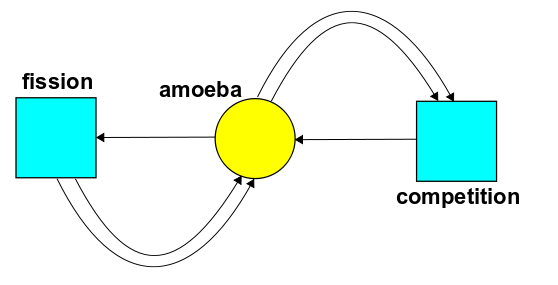
We saw that the rate equation is just the logistic equation, familiar from population biology. The equilibrium solution is complex balanced, because pairs of amoebas are getting created at the same rate as they're getting destroyed, and single amoebas are getting created at the same rate as they're getting destroyed.
So, the Anderson–Craciun–Kurtz theorem guarantees that there's an equilibrium solution of the master equation where the number of amoebas is distributed according to a Poisson distribution. And, we actually checked that this was true!
Next time we'll look at another example.
You can also read comments on Azimuth, and make your own comments or ask questions there!
Here is the answer to the puzzle, provided by David Corfield:
Puzzle. Show that if a classical state $c$ is complex balanced, and we set $x(t) = c$ for all $t,$ then $x(t)$ is a solution of the rate equation.
Answer. Assuming $c$ is complex balanced, we have:
$$ \begin{array}{ccl} \displaystyle{ \sum_{\tau \in T} r(\tau) m(\tau) c^{m(\tau)} } &=& \sum_{\kappa} \sum_{\{\tau : m(\tau) = \kappa\}} r(\tau) m(\tau) c^{m(\tau)} \\ &=& \displaystyle{\sum_{\kappa} \sum_{\{\tau : m(\tau) = \kappa\}} r(\tau) \kappa c^{m(\tau)} } \\ &=& \displaystyle{ \sum_{\kappa} \sum_{\{\tau : n(\tau) = \kappa\}} r(\tau) \kappa c^{m(\tau)} } \\ &=& \displaystyle{ \sum_{\kappa} \sum_{\{\tau : n(\tau) = \kappa\}} r(\tau) n(\tau) c^{m(\tau)}} \\ &=& \displaystyle{\sum_{\tau \in T} r(\tau) n(\tau) c^{m(\tau)} } \end{array} $$
So, we have
$$ \displaystyle{\sum_{\tau \in T} r(\tau) \, (n(\tau) - m(\tau)) \, c^{m(\tau)} = 0 } $$
and thus if $x(t) = c$ for all $t$ then $x(t)$ is a solution of the rate equation:$$ \displaystyle{ \frac{d x}{d t} = 0 = \sum_{\tau \in T} r(\tau)\, (n(\tau)-m(\tau)) \, x^{m(\tau)} } $$
|
|
|
|