


|
|
|
|
This week I want to list a bunch of recent papers and books on n-categories. Then I'll tell you about a conference on the math of environmental sustainability and green technology. And then I'll continue my story about electrical circuits. But first...
This column started with some vague dreams about n-categories and physics. Thanks to a lot of smart youngsters - and a few smart oldsters - these dreams are now well on their way to becoming reality. They don't need my help anymore! I need to find some new dreams. So, "week300" will be the last issue of This Week's Finds in Mathematical Physics.
I still like learning things by explaining them. When I start work at the Centre for Quantum Technologies this summer, I'll want to tell you about that. And I've realized that our little planet needs my help a lot more than the abstract structure of the universe does! The deep secrets of math and physics are endlessly engrossing - but they can wait, and other things can't. So, I'm trying to learn more about ecology, economics, and technology. And I'd like to talk more about those.
So, I plan to start a new column. Not completely new, just a bit different from this. I'll call it This Week's Finds, and drop the "in Mathematical Physics". That should be sufficiently vague that I can talk about whatever I want.
I'll make some changes in format, too. For example, I won't keep writing each issue in ASCII and putting it on the usenet newsgroups. Sorry, but that's too much work.
I also want to start a new blog, since the n-Category Cafe is not the optimal place for talking about things like the melting of Arctic ice. But I don't know what to call this new blog - or where it should reside. Any suggestions?
I may still talk about fancy math and physics now and then. Or even a lot. We'll see. But if you want to learn about n-categories, you don't need me. There's a lot to read these days. I mentioned Carlos Simpson's book in "week291" - that's one good place to start. Here's another introduction:
1) John Baez and Peter May, Towards Higher Categories, Springer, 2009. Also available at http://ncatlab.org/johnbaez/show/Towards+Higher+Categories
This has a bunch of papers in it, namely:
After browsing these, you should probably start studying (∞,1)-categories, which are ∞-categories where all the n-morphisms for n > 1 are invertible. There are a few different approaches, but luckily they're nicely connected by some results described in Julia Bergner's paper. Two of the most important approaches are "Segal spaces" and "quasicategories". For the latter, start here:
2) Andre Joyal, The Theory of Quasicategories and Its Applications, http://www.crm.cat/HigherCategories/hc2.pdf
and then go here:
3) Jacob Lurie, Higher Topos Theory, Princeton U. Press, 2009. Also available at http://www.math.harvard.edu/~lurie/papers/highertopoi.pdf
This book is 925 pages long! Luckily, Lurie writes well. After setting up the machinery, he went on to use (∞,1)-categories to revolutionize algebraic geometry:
4) Jacob Lurie, Derived algebraic geometry I: stable infinity-categories,
available as arXiv:math/0608228.
Derived algebraic geometry II: noncommutative algebra, available as
arXiv:math/0702299.
Derived algebraic geometry III: commutative algebra, available as
arXiv:math/0703204.
Derived algebraic geometry IV: deformation theory, available as
arXiv:0709.3091.
Derived algebraic geometry V: structured spaces, available as
arXiv:0905.0459.
Derived algebraic geometry VI: Ek algebras, available as arXiv:0911.0018.
For related work, try these:
5) David Ben-Zvi, John Francis and David Nadler, Integral transforms and Drinfeld centers in derived algebraic geometry available as arXiv:0805.0157.
6) David Ben-Zvi and David Nadler, The character theory of a complex group, available as arXiv:0904.1247.
Lurie is now using (∞,n)-categories to study topological quantum field theory. He's making precise and proving some old conjectures that James Dolan and I made:
7) Jacob Lurie, On the classification of topological field theories, available as arXiv:0905.0465.
Jonathan Woolf is doing it in a somewhat different way, which I hope will be unified with Lurie's work eventually:
8) Jonathan Woolf, Transversal homotopy theory, available as arXiv:0910.3322.
All this stuff is starting to transform math in amazing ways. And I hope physics, too - though so far, it's mainly helping us understand the physics we already have.
Meanwhile, I've been trying to figure out something else to do. Like a lot of academics who think about beautiful abstractions and soar happily from one conference to another, I'm always feeling a bit guilty, wondering what I could do to help "save the planet". Yes, we recycle and turn off the lights when we're not in the room. If we all do just a little bit... a little will get done. But surely mathematicians have the skills to do more!
But what?
I'm sure lots of you have had such thoughts. That's probably why Rachel Levy ran this conference last weekend:
9) Conference on the Mathematics of Environmental Sustainability and Green Technology, Harvey Mudd College, Claremont, California, Friday-Saturday, January 29-30, 2010. Organized by Rachel Levy.
Here's a quick brain dump of what I learned.
First, Harry Atwater of Caltech gave a talk on photovoltaic solar power:
10) Atwater Research Group, http://daedalus.caltech.edu/
The efficiency of silicon crystal solar cells peaked out at 24% in 2000. Fancy "multijunctions" get up to 40% and are still improving. But they use fancy materials like gallium arsenide, gallium indium phosphide, and rare earth metals like tellurium. The world currently uses 13 terawatts of power. The US uses 3. But building just 1 terawatt of these fancy photovoltaics would use up more rare substances than we can get our hands on:
11) Gordon B. Haxel, James B. Hedrick, and Greta J. Orris, Rare earth elements - critical resources for high technology, US Geological Survey Fact Sheet 087-02, available at http://pubs.usgs.gov/fs/2002/fs087-02/
So, if we want solar power, we need to keep thinking about silicon and use as many tricks as possible to boost its efficiency.
There are some limits. In 1961, Shockley and Quiesser wrote a paper on the limiting efficiency of a solar cell. It's limited by thermodynamical reasons! Since anything that can absorb energy can also emit it, any solar cell also acts as a light-emitting diode, turning electric power back into light:
12) W. Shockley and H. J. Queisser, Detailed balance limit of efficiency of p-n junction solar cells, J. Appl. Phys. 32 (1961) 510-519.
13) Wikipedia, Schockley-Quiesser limit, http://en.wikipedia.org/wiki/Shockley%E2%80%93Queisser_limit
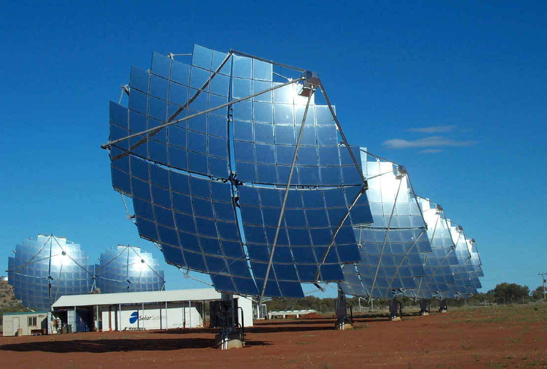
What are the tricks used to approach this theoretical efficiency? Multijunctions use layers of different materials to catch photons of different frequencies. The materials are expensive, so people use a lens to focus more sunlight on the photovoltaic cell. The same is true even for silicon - see the Umuwa Solar Power Station in Australia. But then the cells get hot and need to be cooled.
Roughening the surface of a solar cell promotes light trapping, by large factors! Light bounces around ergodically and has more chances to get absorbed and turned into useful power. There are theoretical limits on how well this trick works. But those limits were derived using ray optics, where we assume light moves in straight lines. So, we can beat those limits by leaving the regime where the ray-optics approximation holds good. In other words, make the surface complicated at length scales comparable to the wavelength at light.
For example: we can grow silicon wires from vapor! They can form densely packed structures that absorb more light:
14) B. M. Kayes, H. A. Atwater, and N. S. Lewis, Comparison of the device physics principles of planar and radial p-n junction nanorod solar cells, J. Appl. Phys. 97 (2005), 114302.
James R. Maiolo III, Brendan M. Kayes, Michael A. Filler, Morgan C. Putnam, Michael D. Kelzenberg, Harry A. Atwater and Nathan S. Lewis, High aspect ratio silicon wire array photoelectrochemical cells, J. Am. Chem. Soc. 129 (2007), 12346-12347.
Also, with such structures the charge carriers don't need to travel so far to get from the n-type material to the p-type material. This also boosts efficiency.
There are other tricks, still just under development. Using quasiparticles called "surface plasmons" we can adjust the dispersion relations to create materials with really low group velocity. Slow light has more time to get absorbed! We can also create "meta-materials" whose refractive index is really wacky - like n = -5!
I should explain this a bit, in case you don't understand. Remember, the refractive index of a substance is the inverse of the speed of light in that substance - in units where the speed of light in vacuum equals 1. When light passes from material 1 to material 2, it takes the path of least time - at least in the ray-optics approximation. Using this you can show Snell's law:
sin(θ1)/sin(θ2) = n2/n1
where ni is the index of refraction in the ith material and θi is the angle between the light's path and the line normal to the interface between materials:
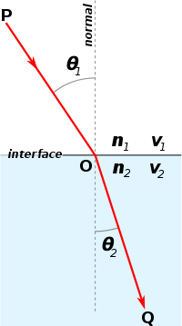
Air has an index of refraction close to 1. Glass has an index of refraction greater than 1. So, when light passes from air to glass, it "straightens out": its path becomes closer to perpendicular to the air-glass interface. When light passes from glass to air, the reverse happens: the light bends more. But the sine of an angle can never exceed 1 - so sometimes Snell's law has no solution. Then the light gets stuck! More precisely, it's forced to bounce back into the glass. This is called "total internal reflection", and the easiest way to see it is not with glass, but water. Dive into a swimming pool and look up from below. You'll only see the sky in a limited disk. Outside that, you'll see total internal reflection.
Okay, that's stuff everyone learns in optics. But negative indices of refraction are much weirder! The light entering such a material will bend backwards.

Materials with a negative index of refraction also exhibit a reversed version of the ordinary Goos-Hänchen effect. In the ordinary version, light "slips" a little before reflecting during total internal reflection. The "slip" is actually a slight displacement of the light's wave crests from their expected location - a "phase slip". But for a material of negative refractive index, the light slips backwards. This allows for resonant states where light gets trapped in thin films. Maybe this can be used to make better solar cells.
Next, Kenneth Golden gave a talk on sea ice, which covers 7-10% of the ocean's surface and is a great detector of global warming. He's a mathematician at the University of Utah who also does measurements in the Arctic and Antarctic. If you want to go to math grad school without becoming a nerd - if you want to brave 70-foot swells, dig trenches in the snow and see emperor penguins - you want Golden as your advisor:
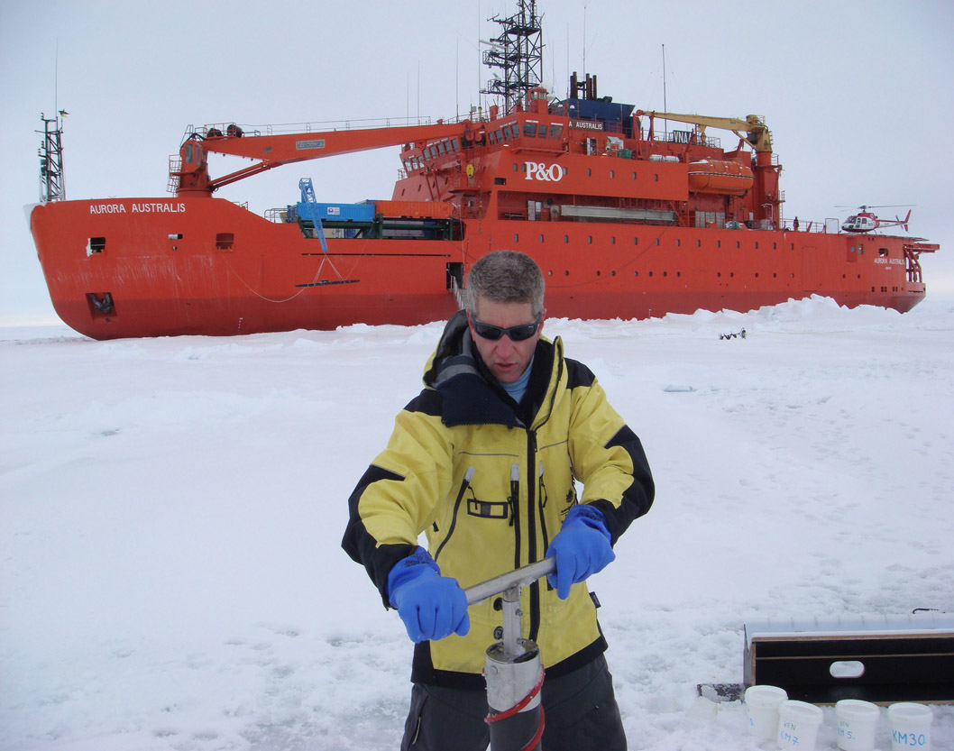
15) Ken Golden's website, http://www.math.utah.edu/~golden/
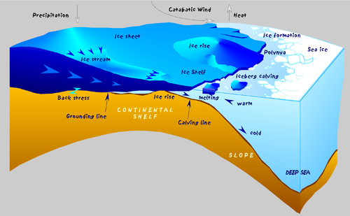
Salt gets incorporated into sea ice via millimeter-scale brine inclusions between ice platelets, forming a "dendritic platelet structure". Melting sea ice forms fresh water in melt ponds atop the ice, while the brine sinks down to form "bottom water" driving the global thermohaline conveyor belt. You've heard of the Gulf Stream, right? Well, that's just part of this story.
When it gets hotter, the Earth's poles get less white, so they absorb more light, making it hotter: this is "ice albedo feedback". Ice albedo feedback is largely controlled by melt ponds. So if you're interested in climate change, questions like the following become important: when do melt ponds get larger, and when do they drain out?
Sea ice is diminishing rapidly in the Arctic - much faster than all the existing climate models had predicted. In the Arctic, winter sea ice diminished in area by about 10% from 1978 to 2008. But summer sea ice diminished by about 40%! It took a huge plunge in 2007, leading to a big increase in solar heat input due to the ice albedo effect.
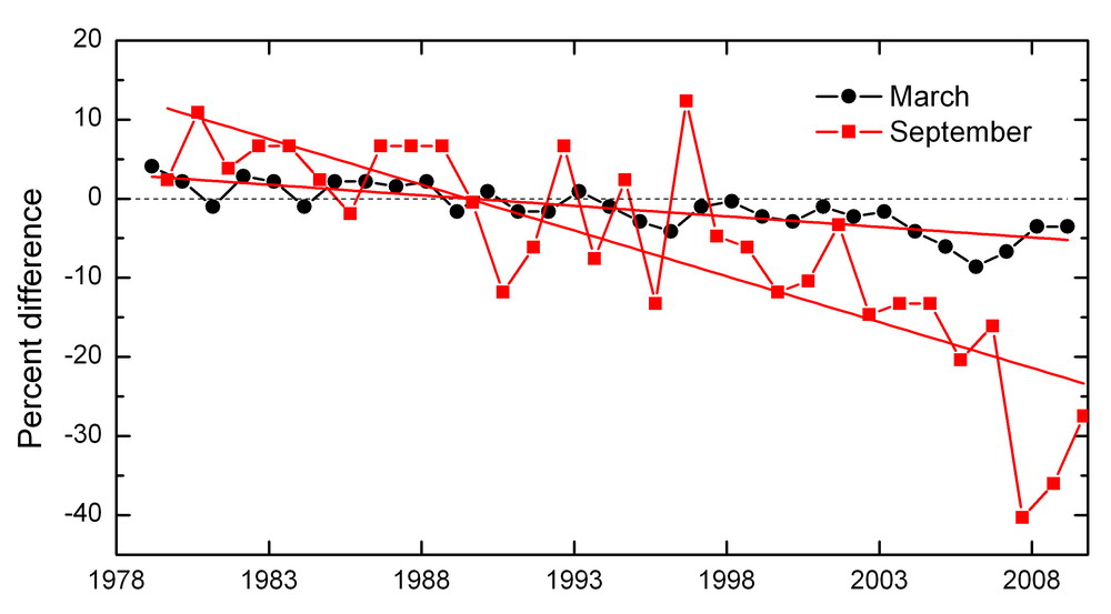
16) Donald K. Perovich, Jacqueline A. Richter-Menge, Kathleen F. Jones, and Bonnie Light, Sunlight, water, and ice: Extreme Arctic sea ice melt during the summer of 2007, Geophysical Research Letters, 35 (2008), L11501. Also available at http://www.crrel.usace.army.mil/sid/personnel/perovichweb/index1.htm
There's a lot less sea ice in the Antarctic than in the Arctic. Most of it is the Weddell Sea, and there it seems to be growing, maybe due to increased precipitation.
There's a lot of interesting math involved in understanding the dynamics of sea ice. The ice thickness distribution equation was worked out by Thorndike et al in 1975. The heat equation for ice and snow was worked out by Maykut and Understeiner in 1971. Sea ice dynamics was studied by Kibler.
Ice floes have two fractal regimes, one from 1 to 20 meters, another from 100 to 1500 meters. Brine channels have a fractal character well modeled by "diffusion limited aggregation". Brine starts flowing when there's about 5% of brine in the ice - a kind of percolation problem familiar in statistical mechanics. Here's what it looks like when there's 5.7% brine and the temperature is -8 °C:
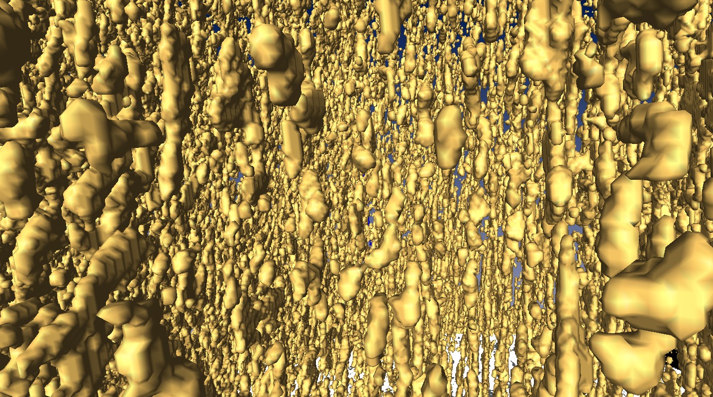
17) Kenneth Golden, Brine inclusions in a crystal of lab-grown sea ice, http://www.math.utah.edu/~golden/7.html
Nobody knows why polycrystalline metals have a log-normal distribution of crystal sizes. Similar behavior, also unexplained, is seen in sea ice.
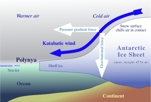
A "polynya" is an area of open water surrounded by sea ice. Polynyas occupy just .001% of the overall area in Antarctic sea ice, but create 1% of the icea. Icy cold katabatic winds blow off the mainland, pushing away ice and creating patches of open water which then refreeze.
There was anomalous export of sea ice through Fran Strait in the 1990s, which may have been one of the preconditions for high ice albedo feedback.
20-40% of sea ice is formed by surface flooding followed by refreezing. This was not included in the sea ice models that gave such inaccurate predictions.
The food chain is founded on diatoms. These form "extracellular polymeric substances"- goopy mucus-like stuff made of polysaccharides that protects them and serves as antifreeze. There's a lot of this stuff; the ice gets visibly stained by it.
For more, see:
18) Kenneth M. Golden, Climate change and the mathematics of transport in sea ice, AMS Notices, May 2009. Also available at http://www.ams.org/notices/200905/
19) Mathematics Awareness Month, April 2009: Mathematics and Climate, http://www.mathaware.org/mam/09/
Next, Julie Lundquist, who just moved from Lawrence Livermore Labs to the University of Colorado, spoke about wind power:
20) Julie Lunquist, Department of Atmospheric and Oceanic Sciences, University of Colorado, http://paos.colorado.edu/people/lundquist.php
With increased reliance on wind, the power grid will need to be redesigned to handle fluctuating power sources. In the US, currently, companies aren't paid for power they generate in excess of the amount they promised to make. So, accurate prediction is a hugely important game. Being off by 1% can cost millions of dollars! Europe has different laws, which encourage firms to maximize the amount of wind power they generate.
If you had your choice about where to build a wind turbine, you'd build it on the ocean or a very flat plain, where the air flows rather smoothly. Hilly terrain leads to annoying turbulence - but sometimes that's your only choice. Then you need to find the best spots, where the turbulence is least bad. Complete simulation of the Navier-Stokes equations is too computationally intensive, so people use fancier tricks. There's a lot of math and physics here.
For weather reports people use "mesoscale simulation" which cleverly treats smaller-scale features in an averaged way - but we need more fine-grained simulations to see how much wind a turbine will get. This is where "large eddy simulation" comes in. Eddy diffusivity is modeled by Monin-Obukhov similarity theory:
21) American Meteorological Society Glossary, Monin-Obukhov similarity theory, http://amsglossary.allenpress.com/glossary/search?id=monin-obukhov-similarity-theory1
A famous Brookhaven study suggested that the power spectrum of wind has peaks at 4 days, 1/2 day, and 1 minute. This perhaps justifies an approach where different time scales, and thus length scales, are treated separately and the results then combined somehow. The study is actually a bit controversial. But anyway, this is the approach people are taking, and it seems to work.
Night air is stable - but day air is often not, since the ground is hot, and hot air rises. So when a parcel of air moving along hits a hill, it can just shoot upwards, and not come back down! This means lots of turbulence.
The wind turbines at Altamont Pass in California kill more raptors than all other wind farms in the world combined! Old-fashioned wind turbines look like nice places to perch, spelling death to birds. Cracks in concrete attract rodents, which attract raptors, who get killed. The new ones are far better.
For more:
22) National Renewable Energy Laboratory, Research needs for winds resource characterization, available as http://www.nrel.gov/docs/fy08osti/43521.pdf
Finally, there was a talk by Ron Lloyd of Fat Spaniel Technologies. This is a company that makes software for solar plants and other sustainable energy companies:
23) Fat Spaniel Technologies, http://www.fatspaniel.com/products/
His talk was less technical so I didn't take detailed notes. One big point I took away was this: we need better tools for modelling! This is especially true with the coming of the "smart grid". In its simplest form, this is a power grid that uses lots of data - for example, data about power generation and consumption - to regulate itself and increase efficiency. Surely there will be a lot of math here. Maybe even the topic I've been talking about lately: bond graphs!
But now I want to talk about some very simple aspects of electrical circuits. Last week I listed various kinds of circuits. Now let's go into a bit more detail - starting with the simplest kind: circuits made of just wires and linear resistors, where the currents and voltages are independent of time.
Mathematically, such a circuit is a graph equipped with some extra data. First, each edge has a number associated to it - the "resistance". For example:
               o----1----o----3----o
               |         |         |
               |         |         |
               2         3         2
               |         |         |
               |         |         |
               o----3----o----1----o
Second, we have current flowing through this circuit. To describe this,
we first arbitrarily pick an orientation on each edge:
               o---->----o---->----o
               |         |         |
               |         |         |
               V         V         V
               |         |         |
               |         |         |
               o----<----o---->----o
Then we label each edge with a number saying how much "current"
is flowing through that edge, in the direction of the arrow:
                    2        3
               o---->----o---->----o
               |         |         |
               |         |         |
             3 V         V 1       V 3
               |         |         |
               |         |         |
               o----<----o---->----o
                    2       -3
Electrical engineers call the current I. Mathematically it's good
to think of I as a "1-chain": a formal linear combination of
oriented edges of our graph, with the coefficients of the linear combination
being the numbers shown above.
If we know the current, we can work out a number for each vertex of our graph, saying how much current is flowing out of that vertex, minus how much is flowing in:
                         2
             5 o---->----o---->----o 0
               |         |         |
               |         |         |
               V         V         V
               |         |         |
               |         |         |
            -5 o----<----o---->----o 0
                       -2
Mathematically we can think of this as a "0-chain": a formal
linear combination of the vertices of our graph, with the numbers
shown above as coefficients. We call this 0-chain the
"boundary" of the 1-chain we started with. Since our
current was called I, we call its boundary δI.
Kirchhoff's current law says that
δI = 0
When this holds, let's say our circuit is a "closed". Physically this follows from the law of conservation of electrical charge, together with a reasonable assumption. Current is the flow of charge. If the total current flowing into a vertex wasn't equal to the amount flowing out, charge - positive or negative - would be building up there. But for a closed circuit, we assume it's not.
If a circuit is not closed, let's call it "open". These are interesting too. For example, we might have a circuit like this:
               x
               |
               |
               V
               |
               |
               o---->----o
               |         |
               |         |
               V         V
               |         |
               |         |
               x         x
where we have current flowing in the wire on top and flowing out the
two wires at bottom. We allow δI to be nonzero at the ends
of these wires - the 3 vertices labelled x. This circuit is an
"open system" in the sense of "week290", because it has these wires dangling
out of it. It's not self-contained; we can use it as part of some
bigger circuit. We should really formalize this more, but I won't now.
Derek Wise did it more generally here:
24) Derek Wise, Lattice p-form electromagnetism and chain field theory, available as gr-qc/0510033.
The idea here was to get a category where chain complexes are morphisms. In our situation, composing morphisms amounts to gluing the output wires of one circuit into the input wires of another. This is an example of the general philosophy I'm trying to pursue, where open systems are treated as morphisms.
We've talked about 1-chains and 0-chains... but we can also back up and talk about 2-chains! Let's suppose our graph is connected - it is in our example - and let's fill it in with enough 2-dimensional "faces" to get something contractible. We can do this in a god-given way if our graph is drawn on the plane: just fill in all the holes!
               o---------o---------o
               |/////////|/////////|
               |/////////|/////////|
               |//FACE///|///FACE//|
               |/////////|/////////|
               |/////////|/////////|
               o---------o---------o
In electrical engineering these faces are often called
"meshes".
This give us a chain complex
        δ           δ
C0 <-------- C1 <-------- C2
Remember, a "chain complex" is just a bunch of vector spaces Ci and linear maps δ: Ci → Ci-1, obeying the equation δ2 = 0. We also get a cochain complex:
       d           d
C0 --------> C1 ---------> C2
meaning a bunch of vector spaces Ci and linear maps d: Ci → Ci+1, obeying the equation d2 = 0.
As I've already said, it's good to think of the current I as a 1-chain, since then
δI = 0
is Kirchoff's current law. Since our little space is contractible the above equation implies that
I = δJ
for some 2-chain J called the "mesh current". This assigns to each face or "mesh" the current flowing around that face.
An electrical circuit also comes with a third piece of data, which I haven't mentioned yet. Each oriented edge should be labelled by a number called the "voltage" across that edge. Electrical engineers call the voltage V. It's good to think of V as a 1-cochain, which assigns to each edge the voltage across that edge.
Why a 1-cochain instead of a 1-chain? Because then
dV = 0
is the other basic law of electrical circuits - Kirchhoff's voltage law! This law says that the sum of these voltages around a mesh is zero. Since our little space is contractible the above equation implies that
V = dφ
for some 0-cochain φ called the "electrostatic potential". In electrostatics, this potential is a function on space. Here it assigns a number to each vertex of our graph.
Since the space of 1-cochains is the dual of the space of 1-chains, we can take the voltage V and the current I, glom them together, and get a number:
V(I)
This the "power": that is, the rate at which our network soaks up energy and dissipates it into heat. Note that this is just a fancy version of formula for power that I explained in "week290" - power is effort times flow.
I've given you three basic pieces of data labelling our circuit: the resistance R, the current I, and the voltage V. But these aren't independent! Ohm's law says that the voltage across any edge is the current through that times the resistance of that edge. But this remember: current is a 1-chain while voltage is a 1-cochain. So "resistance" can be thought of as a map from 1-chains to 1-cochains:
R: C1 → C1
This lets us write Ohm's law like this:
V = RI
This, in turn, means the power of our circuit is
V(I) = (RI)(I)
For physical reasons, this power is always nonnegative. In fact, let's assume it's positive unless I = 0. This is just another way of saying that resistance labelling each edge is positive. It can be very interesting to think about circuits with perfectly conducting wires. These would give edges whose resistance is zero. But that's a bit of an idealization, and right now I'd rather allow only positive resistances.
Why? Because then we can think of the above formula as the inner product of I with itself! In other words, then there's a unique inner product on 1-chains with
(RI)(I) = <I,I>
In this situation
R: C1 → C1
is the usual isomorphism that we get between a finite-dimensional inner product space and its dual. (For this statement to be true, we'd better assume our graph has finitely many vertices and edges.)
Now, if you've studied de Rham cohomology, all this should start reminding you of Hodge theory. And indeed, it's a baby version of that! So, we're getting a little bit of Hodge theory, but in a setting where our chain complexes are really morphisms in a category. Or more generally, n-morphisms in an n-category!
There's a lot more to say, but that's enough for now. Here are some references on "electrical circuits as chain complexes":
25) Paul Bamberg and Shlomo Sternberg, A Course of Mathematics for Students of Physics, Cambridge University, Cambridge, 1982.
Bamberg and Sternberg is a great book overall for folks wanting to get started on mathematical physics. The stuff about circuits starts in chapter 12.
26) P. W. Gross and P. Robert Kotiuga, Electromagnetic Theory and Computation: A Topological Approach, Cambridge University Press, 2004.
This book says just a little about electrical circuits of the sort we're discussing, but it says a lot about chain complexes and electromagnetism. It's a great place to start if you know some electromagnetism but have never seen a chain complex.
Addenda: I thank Colin Backhurst, G.R.L. Cowan, David Corfield, Mikael Vejdemo Johansson and Tim Silverman for corrections. I thank Garett Leskowitz for pointing out the material in Bamberg and Sternberg's book.
Ed Allen writes:
Regarding the silicon technologies for improving efficiency of light capture, the Mazur lab's black silicon projects are something I've been following for a few years:27) Mazur Group, Optical hyperdoping - black silicon, http://mazur-www.harvard.edu/research/detailspage.php?rowid=1
28) Wikipedia, Black silicon, http://en.wikipedia.org/wiki/Black_silicon
29) Anne-Marie Corley, Pink silicon is the new black, Technology Review, Thursday, July 9, 2009. Also available at http://www.technologyreview.com/computing/22975/?a=f
David Corfield wonders if it's really true that there's a lot less sea ice in the Antarctic than the Arctic:
Was that right? Cryosphere has the Arctic sea ice oscillating on average between 5 and 14 million sq km, and the Antarctic between 2 and 15 million sq km.Recently of course that 5 has become 3.
Best, David
For more discussion, visit the n-Category Café.
So many young people are forced to specialize in one line or another that a young person can't afford to try and cover this waterfront - only an old fogy who can afford to make a fool of himself. If I don't, who will? - John Wheeler
© 2010 John Baez
baez@math.removethis.ucr.andthis.edu
|
|
|
|