


|
|
|
|
I have a lot to talk about, since I just got back from this quantum gravity summer school in Corfu:
1) 2nd School and workshop on quantum gravity and quantum geometry, September 13-20, 2009, organized by John Barrett, Harald Grosse, Larisa Jonke and George Zoupanos. Information at http://www.physics.ntua.gr/corfu2009/qg.html
I felt a bit like Rip Van Winkle, the character who fell asleep for 20 years and woke to find everything changed. I gave up working on quantum gravity about 4 years ago because so many problems seemed intractable. Now a lot of these have been solved, or at least seen some progress. It was great!
The school featured courses by Ashtekar, Barrett, Rivasseau, Rovelli and myself - we each gave 5 hours of lectures. All these guys were friends whom I was very happy to see again - except for Rivasseau, whom I'd never met. But it was great to meet him, since he works on mathematically rigorous quantum field theory, the topic I tried to do my PhD on. He had some amazing things to say about the combinatorics of trees and the problem of summing divergent series. Sadly, right now I only have time to summarize the courses by Ashtekar and Rovelli.
Abhay Ashtekar gave a review of recent work on loop quantum cosmology. Starting with the work of Martin Bojowald around 2001, there's been a lot of interest in the possibility that loop quantum gravity could eliminate the singularity at the Big Bang. The big problem is that dynamics in loop quantum gravity is not understood. There are lots of choices for how it might work, and nobody knows which is right, or if there even is a right one. Luckily, by imposing the symmetry conditions appropriate to a homogeneous isotropic cosmology one can narrow down the problem of seeking a reasonable dynamics to something much more manageable. Instead of infinitely many degrees of freedom, there are just a few.
Unfortunately, there are still lots of choices involved in guessing a reasonable theory of quantum cosmology inspired by loop quantum gravity. Checking their implications involves both computer calculations and conceptual head-scratching. So, it took about 7 years to find a satisfactory candidate. It might not be right, but at least it's self-consistent and elegant. For a nice survey, see this:
2) Abhay Ashtekar, Loop quantum cosmology: an overview, Gen. Rel. Grav. 41 (2009), 707-741. Also available as arXiv:0812.0177.
Section IVa sketches the history of the subject, but it's best to read the previous stuff first.
Anyway, what are the results? What does the currently popular theory of loop quantum cosmology imply?
In a nutshell: if you follow the history of the Universe back in time, it looks almost exactly like what ordinary cosmology predicts until the density reaches about 1/100 of the Planck density.
What's the Planck density, you ask?
Well, you can cook up units of mass, length and time by saying that Planck's constant and the speed of light and Newton's gravitational constant are all 1 in these units. Unsurprisingly, these units are called:
The "Planck density" is one Planck mass per cubic Planck length - or in ordinary units, about 5×1096 kilograms per cubic meter. That's incredibly dense! It's what you'd get by compressing 1023 solar masses into the volume of an atomic nucleus.
According to loop quantum cosmology, at around 1/100 the Planck density quantum gravity effects come in, creating a force that prevents the universe from shrinking further as we march backwards in time. And at about .4 times the Planck density, there's a "bounce". Going further back in time, we see the Universe expand again! Indeed, the Universe is symmetrical in time around the moment of maximum compression.
So, the Big Bang is replaced by a Big Bounce.
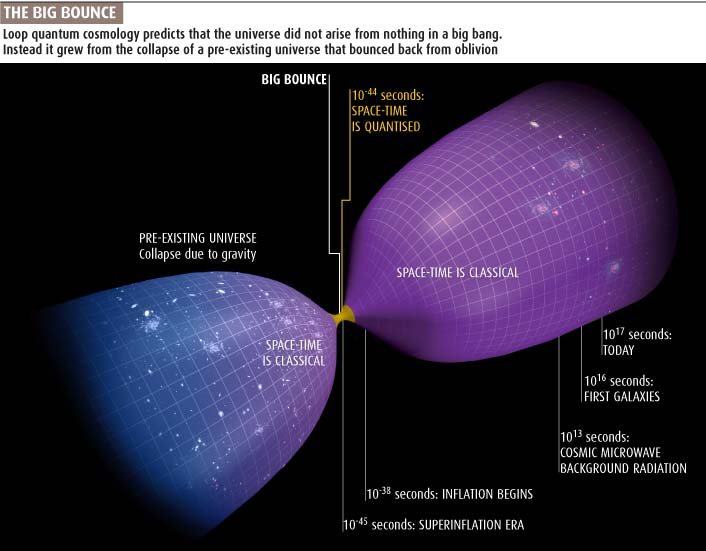
The above picture comes from this popular account:
3) Anil Ananthaswamy, From Big Bang to Big Bounce, New Scientist, December 13, 2008, pp. 32-35. Also available at http://gravity.psu.edu/outreach/articles/bigbounce.pdf
Interestingly, in this model quantum effects don't create much dispersion as the Universe passes through a big bounce. In other words: if the Universe's wavefunction is sharply peaked around a certain classical geometry, it remains so through the big bounce. It doesn't "smear out" too much.
By the way, I would be very happy if anyone working on loop quantum cosmology could give me a intuitive physical explanation for the force that prevents the singularity. Mathematically I know that it arises from a kind of discretization. Instead of talking about the curvature of spacetime at infinitesimally small scales, we can only measure curvature by carrying a particle around a finite-sized loop. This has little effect when spacetime is only slightly curved, but when the curvature is big it makes a big difference. This causes an effect very much like a force that prevents the Universe from crushing down to nothing as we follow it backwards in time.
So far, so good. But a good physical intuition would explain the sign of this effective force. Why does it prevent the singularity instead of, say, making it worse?
For some more details, try this treatment which resembles the course Ashtekar taught:
4) Abhay Ashtekar, An introduction to loop quantum gravity through cosmology, Nuovo Cimento 122B (2007), 135-155. Also available as arXiv:gr-qc/0702030.
Anyway, the real fun will start when people systematically compute the behavior of inhomogeneous perturbations in loop quantum cosmology model. After all, the little ripples in the microwave background radiation are the first interesting thing we see in the Universe.
A lot of work on cosmology studies these inhomogeneities by calculating backwards to a hypothesized "inflationary epoch" about 10-35 seconds after the Big Bang - or Big Bounce, if that's your theory. Quantum gravity effects are likely to become important only at much earlier times, since the Planck time is about 10-43 seconds. Here I'm using "much earlier" in a funny logarithmic sense. But that's actually appropriate here. The inflationary epoch comes about 100 million Planck times after the Big Bounce. According to Ashtekar's calculations, by then quantum gravity corrections only affect the rate of expansion of the universe by about one part in 100 thousand. So, it's not clear that loop quantum gravity calculations are going to have anything interesting to say about anything we can see today. But who knows?
Next, Carlo Rovelli. His class was an introduction to spin foam models, which are an attempt to pin down a specific dynamics for loop quantum gravity. Here I'm going to get more technical, because this material is closer to my heart. If you need a warmup, try "week109"-"week113" for the basics.
I worked on spin foams for about 5 years. I love them because they offer the hope of building spacetime from abstract algebra - higher category theory, in fact. But I gave up because a lot of puzzle pieces just didn't seem to be fitting together. Back then, the best candidate for a spin foam model of gravity was the Barrett-Crane model. But there were three big problems:
A) The Barrett-Crane model used spin networks of a different kind from the usual ones in loop quantum gravity. Instead of spin networks with edges labelled by unitary representations of SU(2) (the double cover of the rotation group), it used unitary representations of SL(2,C) (the double cover of the Lorentz group). This is because it's all about spacetime, while loop quantum gravity focuses on space. And instead of using spin networks with vertices labelled by arbitrary intertwiners, it only used a special intertwiner called the "Barrett-Crane intertwiner".B) While loop quantum gravity in its modern formulation includes the Immirzi parameter - a dimensionless constant that sets the scale of area quantization - the Barrett-Crane model did not. If the currently accepted calculations are right, we need to choose a special and rather peculiar value of the Immirzi parameter if we want loop quantum gravity to get the right answer for the entropy of black holes. So, along with problem A), this makes it even harder to connect the Barrett-Crane model to loop quantum gravity.
C) At first people hoped for various clues linking the Barrett-Crane model to general relativity. For example, we hoped that the asymptotic value of the amplitude for a large 4-simplex in the Barrett-Crane model was nicely related to the action for general relativity. But this turned out to be false: in the Barrett-Crane model, the amplitude for a large 4-simplex is dominated by certain degenerate geometries where the 4-simplex is squashed down to 3 dimensions. See "week128", "week168", "week170" and "week198" for the story here. Carlo Rovelli raised our hopes again in a more sophisticated way: he tried to compute the propagator for gravitons starting from the Barrett-Crane model. For a beautiful and physically very sensible reason, the degenerate geometries don't dominate this calculation. Rovelli got some promising results for certain components of the graviton propagator, and left a student to work out the rest of the components... but it didn't work!
It seems all these problems have been solved now. There's a new model sometimes called the EPRL model, after Engle, Pereira, Rovelli, and Livine, although other people were involved as well - I'll list some papers later.
The basic idea of the EPRL model is to start with the Holst Lagrangian for general relativity. In 1995, Soren Holst came up with a nice Lagrangian for gravity:
5) Soren Holst, Barbero's Hamiltonian derived from a generalized Hilbert-Palatini action, Phys. Rev. D53 (1996), 5966-5969. Also available as arXiv:gr-qc/9511026.
It looks like this:
tr(e ^ e ^ *F) + (1/γ) tr(e ^ e ^ F)
I'll explain this in detail later, because there was a student who twice asked about the math behind this Lagrangian, and Rovelli and I brushed the question off by saying "it's just like Palatini Lagrangian". I feel guilty, so someone find that student and tell him to read my explanation below.
But that gets a bit technical, so for now let me say: "it's just like the Palatini Lagrangian". Namely, the first term is the usual Palatini Lagrangian for gravity. The second term involves the Immirzi parameter, γ. The second term doesn't affect the classical equations of motion, because its variation is a total derivative. But it does affect the quantum theory!
If we triangulate spacetime and carry out a spin foam quantization of this theory - which is a bit like doing lattice gauge theory - we can show (in a rough-and-ready physicist's way) that the partition function of the quantum theory is computed as a sum over spin foams where the spin foams are labelled by certain special representations of SL(2,C).
Physicists don't learn the unitary representations of the Lorentz group in school the way they do for the Poincare group. But the unitary representations of the Lorentz group - or its double cover SL(2,C) - are very nice. Except for the trivial representation they're all infinite-dimensional, which is a bit scary at first... but there's a bunch called the "principal series" indexed by a spin j = 0,1/2,1,3/2,... and a nonnegative real number I'll call k. Very roughly speaking the spin j has to do with rotations, while k is an analogous quantity related to boosts. If you want more details, the only online explanation I can find is this:
6) Wikipedia, Representation theory of the Lorentz group, http://en.wikipedia.org/wiki/Representation_theory_of_the_Lorentz_group
It may be better to read some of the many books cited there.
Anyway, the special representations of SL(2,C) that show up in the EPRL model are those with
k = γ j
This is beautiful because there's one for each spin. So, the category of these representations and their direct sums is equivalent to the category of finite-dimensional unitary representations of SU(2)!
This is how the EPRL model gets around problem A) listed above. Spin networks in this new model are nicely compatible with spin networks in loop quantum gravity, because you can think of their edges either as labelled by special representations of SL(2,C), or as labelled by arbitrary representations of SU(2). The first is the "spacetime" or Lagrangian viewpoint, the second is the "space" or Hamiltonian viewpoint.
This is also the key to how the EPRL model gets around problem B). The Immirzi parameter is built into the model in a very natural way. As a result, the quantization of area and volume in this model is compatible with that in loop quantum gravity.
I don't think I'll describe the rest of the model, which consists of a formula for computing the amplitude for a 4-simplex with edges labelled by spins. But it's this formula that solves problem C). The EPRL model gets the graviton propagator right!
Of course there are even bigger tests still ahead for this spin foam model. We need to see if it reduces to general relativity in the classical limit. In other words, we need to get Einstein's equations out of it. And we need to see if it reduces to the usual perturbative theory of quantum gravity in some other limit. In other words, we need to compute, not just graviton propagators (which describe the probability of a lone graviton zipping from here to there on the background of Minkowski spacetime), but graviton scattering amplitudes (which describe the probability of various outcomes when two or more gravitons collide).
Both these tasks are both computationally and conceptually difficult. In other words, it's not just hard to do the calculations: it's hard to know what calculations to do! When I said "in some limit" and "in some other limit", I know what limits these are in a physical sense, but not how to describe them using spin foams. Actually we seem closer to understanding graviton scattering amplitudes, thanks to the work of Rovelli. But it seems miraculous and strange that we can compute graviton propagators (much less scattering amplitudes) using very simple spin foams, as Rovelli and his collaborators have done. Every time I meet him, I ask Rovelli what's going on here: how we can describe the behavior of a graviton in terms of just a few 4-simplices of spacetime.
So, the road is still long, steep, and fraught with danger. But three problems that had everyone completely stumped have now been solved in one elegant blow.
Though there's much more to say, it's dinnertime now. So, let me list some references and then explain the differential geometry behind the Holst Lagrangian, just to make up for not explaining it to that student.
The original "EPR model" was introduced here - but this treated Riemannian rather than Lorentzian metrics, and only in the special case where the second term in the Holst action was left out - so, no Immirzi parameter:
7) Jonathan Engle, Roberto Pereira and Carlo Rovelli, Flipped spinfoam vertex and loop gravity, Nucl. Phys. B798 (2008), 251-290. Also available as arXiv:0708.1236.
This is a very nice paper which describes a lot of geometry that I haven't had time to mention. However, the full-fledged model appeared later:
8) Jonathan Engle, Etera Livine, Roberto Pereira, and Carlo Rovelli, LQG vertex with finite Immirzi parameter, Nucl. Phys. B799 (2008), 136-149. Also available as arXiv:0711.0146.
But there are also other people whose work deserves credit! For example, my friends Laurent Freidel and Kirill Krasnov:
9) Laurent Freidel and Kirill Krasnov, A new spin foam model for 4d gravity, Class. Quant. Grav. 25 (2008), 125018. Also available as arXiv:0708.1595.
This paper gives a bit of the history, which I don't know very well, since I wasn't paying attention. Kirill visited me once and tried to get me interested in his new spin foam model, but I wasn't in the mood. Now that everything is nicely polished, of course I like it more.
There are probably lots of other important papers that I'm leaving out, but let me turn to a few papers that discuss graviton propagators.
Here's the paper where Rovelli's student found problems with getting the graviton propagator from the Barrett-Crane model:
10) Emanuele Alesci and Carlo Rovelli, The complete LQG propagator: I. Difficulties with the Barrett-Crane vertex. Phys. Rev. D76 (2007), 104012. Also available as arXiv:0708.0883.
Then Rovelli and collaborators found numerical evidence that the EPR model seemed to be working better:
11) Elena Magliaro, Claudio Perini and Carlo Rovelli, Numerical indications on the semiclassical limit of the flipped vertex, Class. Quant. Grav. 25 (2008), 095009. Also available as arXiv:0710.5034.
Then Alesci and Rovelli wrote a paper using the new model:
12) Emanuele Alesci and Carlo Rovelli, The complete LQG propagator: II. Asymptotic behavior of the vertex, Phys. Rev. D77 (2008), 044024. Also available as arXiv:0711.1284.
and then Alesci and Rovelli wrote another paper in their series, with Eugenio Bianchi:
13) Emanuele Alesci, Eugenio Bianchi, Carlo Rovelli, LQG propagator: III. The new vertex, available as arXiv:0812.5018.
This paper used the work of John Barrett and collaborators, who analyzed the asymptotics of the amplitude for a 4-simplex in the new model:
14) John W. Barrett, R. J. Dowdall, Winston J. Fairbairn, Henrique Gomes and Frank Hellmann, Asymptotic analysis of the EPRL four-simplex amplitude, available as arXiv:0902.1170.
For a nice treatment of spin foams that generalizes the new model to spin foams that don't come from triangulations of spacetime, try:
15) Wojciech Kaminski, Marcin Kisielowski, Jerzy Lewandowski, Spin-foams for all loop quantum gravity, available as arXiv:0909.0939.
Everything Lewandowski does is very precise, so if you're a mathematician you might actually want to start here.
There are also lots of other papers in this general line of work. I apologize to everyone whose work I didn't cite - like Dan Christensen and Igor Khavkine, for example!
Anyway, I'm excited about this new work and I hope to write another paper or two about spin foam models. I came up with two fun ideas during the Corfu summer school, which I'd like to work on.
But let me conclude by explaining the Holst Lagrangian for gravity. I explained the Palatini Lagrangian and a whole bunch of other Lagrangians for gravity back in "week176". But maybe you were just a kid back then... or maybe you weren't paying adequate attention! So, let me repeat my explanation in slightly different words.
Assume spacetime is an orientable smooth 4-manifold M. Pick a vector bundle T that's isomorphic to the tangent bundle TM. Physicists don't have a name for this bundle, but they call any of its fibers the "internal space". I call it the "fake tangent bundle".
We then equip T with a Lorentzian metric and orientation. This lets us describe a Lorentzian metric on M using a vector bundle map
e: TM → T
This map has lots of names: the "cotetrad", the "soldering form", or the "coframe field". Whatever we call it, we can use it to pull the metric on T back to the tangent bundle. If e is an isomorphism, this gives a Lorentzian metric on M. If it's not, we get something like a metric, but with degenerate directions. For now let's only consider the case where e is an isomorphism.
The cotetrad is one of the two basic fields used to define the Holst action. The other is a metric-compatible connection on T. This connection is usually denoted A and called a "Lorentz connection". Its curvature is denoted F.
Now, what does the Holst Lagrangian
tr(e ^ e ^ *F) + (1/γ) tr(e ^ e ^ F)
actually mean?
First of all, the curvature F is an End(T)-valued 2-form, but using the metric on T we get an isomorphism between T and its dual, so we can also think of the curvature as a 2-form taking values in T tensor T. However, if we do this, the fact that A is metric-compatible means that F is skew-symmetric: it takes values in the second exterior power of T, Λ2(T).
Since T has a metric and orientation, we can define a Hodge star operator on the exterior algebra Λ(T) just as we normally do for differential forms on a manifold with metric and orientation. We call this the "internal" Hodge star operator. Using this we can define *F, which is again a 2-form taking values in Λ2(T).
Next, note that the cotetrad e can be thought of as a T-valued 1-form. This allows us to define the wedge product e ^ e as a Λ2(T)-valued 2-form. This is the same sort of gadget as the curvature F and its internal Hodge dual *F! So, we can take the wedge product of the differential form parts of e ^ e and *F while using the metric on T to pair together their Λ2(T) parts to get a number. The overall result is a plain old 4-form, which we call tr(e ^ e ^ *F). This is the Palatini Lagrangian!
If you work out the equations of motion coming from this Lagrangian, they say A that pulls back via e to a torsion-free metric-compatible connection on the tangent bundle. This is just the Levi-Civita connection! It follows that F pulls back to the curvature of the Levi-Civita connection. This is just the Riemann tensor! Finally, it turns out that tr(e ^ e ^ *F) is just the Ricci scalar curvature times the volume form on M, so we were doing general relativity all along!
We define tr(e ^ e ^ F) the same sort of way, and throwing this term into the action doesn't affect the classical equations of motion. It's very much like Yang-Mills theory, where you can take the usual action
tr(F ^ *F)
and throw in a "theta term", proportional to "second Chern class"
tr(F ^ F)
without changing the classical equations of motion. But it does affect the quantum theory!
For a more detailed treatment of the Holst action including a cosmological constant term proportional to
tr(e ^ e ^ e ^ e)
and three topological terms corresponding to the Pontryagin class, the Euler class and the Nieh-Yan class, see:
16) Danilo Jimenez Rezende and Alejandro Perez, 4d Lorentzian Holst action with topological terms, available as arXiv:0902.3416.
Addenda: I thank Dan Christensen for catching an error in my quick history of the graviton propagator calculations, and Derek Wise for catching some other errors. Urs Schreiber asked a question about how the singularity gets avoided in loop quantum cosmology:
My impression is the following, I'd be grateful to hear what is wrong about it.I replied:What happens is a special case of this: start with a differential equation whose solutions diverge at the origin. Replace it with a difference equation on a subset of points that does not include the origin. This will have solutions not showing the singularity.
This may have been true for some early models - there have been a lot of models between 2001 and now. It's definitely not true for the currently popular models that Ashtekar was explaining.Then Urs asked for more detail, and I admitted that the references given above might not satisfy him:It's true that a differential equation is getting replaced by a difference equation. But the singularity is not being avoided simply by "stepping over it". That would be a cheap trick. In the models under study now, there really is an effective "force" that prevents the singularity. And it arises from the mechanism I sketched:
Instead of talking about the curvature of spacetime at infinitesimally small scales, we can only measure curvature by carrying a particle around a finite-sized loop. This has little effect when spacetime is only slightly curved, but when the curvature is big it makes a big difference. This causes an effect very much like a force that prevents the Universe from crushing down to nothing as we follow it backwards in time.A bit more precisely - but still quite roughly: if the curvature is c, in loop quantum gravity we don't have a quantum operator corresponding to c. Instead we have something more like exp(ic). So we use something like sin(c)=(exp(ic)-exp(-ic))/2i as a substitute for c in certain equations. When the curvature is small these are almost the same. When it gets big, they're different. This gives an effective force that prevents the singularity. This force starts getting big when the density is about 1/100 of the Planck density. When the density hits .41 times the Planck density, it's enough to create a "bounce".
(The math is actually a bit more complicated than what I said, but it's similar in spirit.)
In fact, a bunch of calculations have shown that the quantum dynamics are quite nicely approximated by an "effective Friedmann equation" - a differential equation like the usual classical one that describes the Big Bang, but with an extra term.
And, the solutions of the difference equation are very close to the solutions of this differential equation.
... you might prefer Effective equations for isotropic quantum cosmology including matter by Bojowald, Hernandez and Skirzewski.In Section 2, they start with the Friedmann equation for a homogeneous isotropic cosmology with k=0 and a massless scalar field φ. In Section 2.1 they "deparametrize" this equation, eliminating the time variable by using φ as a clock field, or "internal time" - a standard way of dealing with the problem of time in quantum cosmology. In Section 2.2 they review the standard Wheeler-DeWitt quantization of the resulting theory.
Then, in Section 2.3, they switch to loop quantization. They don't give a vast amount of detail on why one should do this, but they do say what is being done. Briefly, instead of the variable c = da/dτ (the rate of expansion of the universe, closely related to spacetime curvature in this model) we switch to using exp(ic) and exp(-ic). In a deeper treatment this comes from using holonomies instead of the curvature at a point. This is what produces the effective force that prevents the singularity.
They don't derive difference equations in this paper; instead, they just derive effective corrections to the usual Wheeler-DeWitt equation. Calculations have shown that solutions of the resulting differential equations closely match those of the difference equations that a more thorough approach yields. So, as far as physical intuition goes, perhaps the most important thing is to see where these effective corrections to the Wheeler-DeWitt equation come from, and why they prevent the singularity.
For more discussion visit the n-Category Café.
Many fine physicists have burned away their lives grappling with the problem of quantum gravity. - R. P. Woodard
© 2009 John Baez
baez@math.removethis.ucr.andthis.edu
|
|
|
|