 |
 |
Lecture 11 - The Poset of Partitions
Last time we learned about partitions of a set: ways of chopping it into disjoint nonempty sets called "parts".

We also learned about equivalence relations on a set: relations that are reflexive, symmetric and transitive. And we learned that partitions give equivalence relations! If we have a partition of a set, we can decree that two elements of the set are "equivalent" if they are in the same part. For example, any two points in the red part of the picture are equivalent.
Even better, every equivalence relation comes from a unique partition. So, if you want to work with partitions, you can equally well work with equivalence relations. This makes it easy to define a poset of partitions, which is the key step toward doing logic with partitions.
Here's how it goes. For any set \(X\), \( \mathcal{E}(X)\) is the set of partitions of \(X\). For any partition \(P\) of \( X \), let \(\sim_P\) be the corresponding equivalence relation.
Definition. We say that a partition \(P\) of \(X\) is finer than a partition \(Q\) of \(X\) if
[ x \sim_P y \textrm{ implies } x \sim_Q y ]
for all \(x,y \in X \). In this situation we write \(P \le Q\), and we also say \(Q\) is coarser than \(P\).
This makes it incredibly easy to get our hands on the poset of partitions!
Proposition. \((\mathcal{E}(X), \le)\) is a poset.
Proof. We just need to show that the relation \(\le\) is reflexive, transitive and antisymmetric. Since
[ x \sim_P y \textrm{ implies } x \sim_P y ]
for all \(x,y \in X \), we have
[ P \le P ]
so the relation \(\le\) is reflexive.
If
[ x \sim_P y \textrm{ implies } x \sim_Q y ]
and
[ x \sim_Q y \textrm{ implies } x \sim_R y ]
then clearly
[ x \sim_P y \textrm{ implies } x \sim_R y ]
So,
[ P \le Q \textrm{ and } Q \le R \textrm{ implies } P \le R ]
so the relation \(\le\) is transitive.
Finally, to show that \(\le\) is antisymmetric, assume
[ P \le Q \textrm{ and } Q \le P . ]
Then by definition
[ x \sim_P y \textrm{ implies } x \sim_Q y ]
and
[ x \sim_Q y \textrm{ implies } x \sim_P y ]
or in other words,
[ x \sim_P y \textrm{ if and only if } x \sim_Q y. ]
This means that the relations \(\sim_P\) and \(\sim_Q\) are equal, so \(P = Q \) as desired. \( \quad \blacksquare \)
That proof was as easy as slipping down a slide covered with grease! It's what I call a "follow your nose" proof: to create it, you just carefully write down what you need to show, unravel the definitions to figure out what that really means, and notice that it's true.
Here's another way to tell if one partition is finer than another:
Puzzle 34. Given two partitions \(P\) and \(Q\) of a set \(X\), show that \(P \le Q\) if and only if every part of \(P\) is contained in a part of \(Q\).
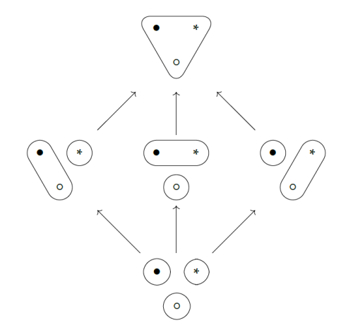
Using this, you can easily work out the poset of partitions of a 3-element set:

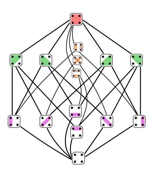
It looks simple. But that's deceptive! For a 4-element set we get this poset of partitions:

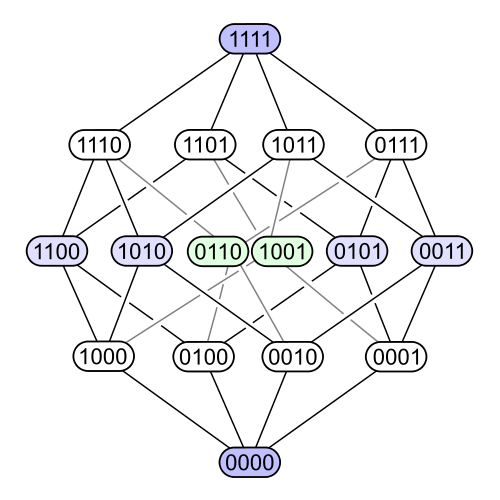
It's much more complicated than the poset of subsets of a 4-element set:

Indeed, there are many difficult questions about the poset of partitions that are easy for the poset of subsets.
For example: how many subsets does an \(n\)-element set have? Easy: \(2^n\). But how many partitions does an \(n\)-element set have? Not so easy: it's the \(n\)th Bell number \(B_n\). The Bell numbers go like this:
[ 1, 1, 2, 5, 15, 52, 203, 877, 4140, 21147, 115975, 678570, \dots ]
Another example: poset of subsets looks the same when you flip it upside down. That's because any subset \(S \subseteq X\) has a complement
[ X - S = \{x \in X : \; x \notin S \} . ]
In the logic of subsets this gives negation: if a subset \(S \subseteq X\) corresponds to some proposition \(P\), its complement \(X - S\) corresponds to the proposition \(\neg P \), which is how logicians write "not \(P\) ".
But the poset of partitions does not look the same when you flip it upside down:

And indeed, there is no "not" in partition logic! It's very different than classical logic. To read more about it, go here:
Partition logic still has joins and meets, so I'll talk about those next time.
We should also see how a function \(f : X \to Y \) gives a monotone function
\(f^* : \mathcal{E}(Y) \to \mathcal{E}(X)\). And we should see if \(f^*\) has left or right adjoints!
This leads up to the punchline of Chapter 1: the idea of "generative effects". In a nutshell, partition logic has "generative effects" because the right adjoint of \(f^*\) doesn't preserve joins. This may sound scary and technical, but as we'll see, it captures a basic fact about reality.
To read other lectures go here.
 |
 |