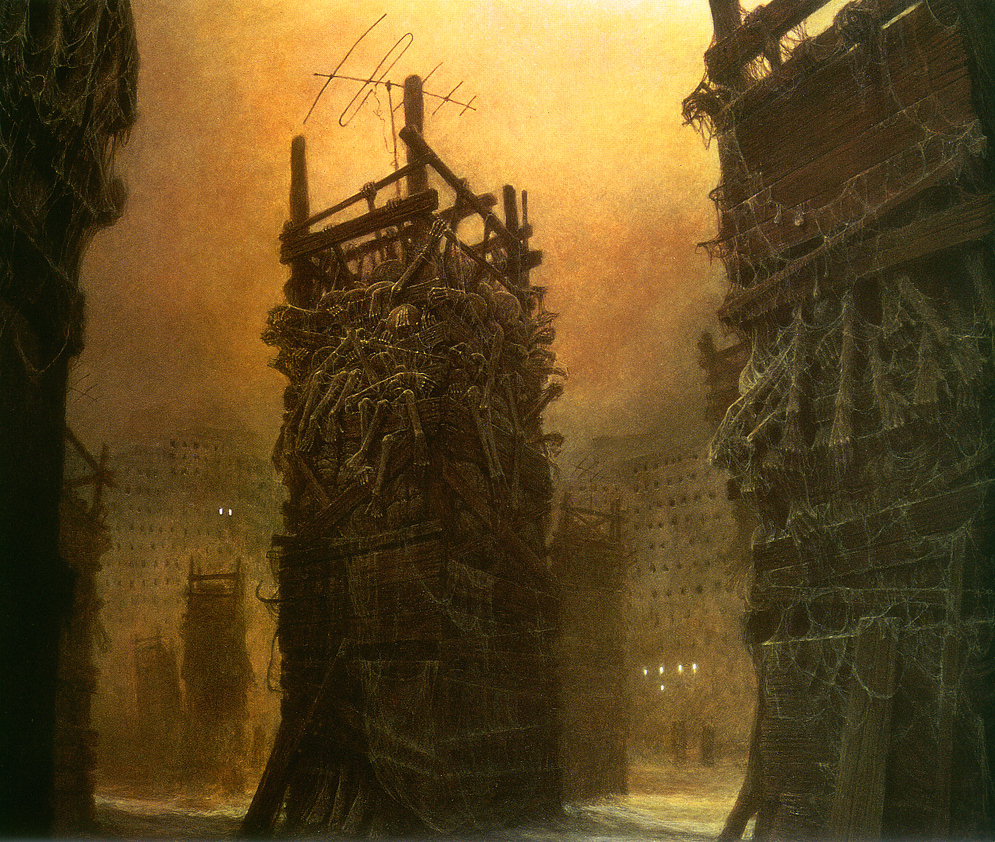
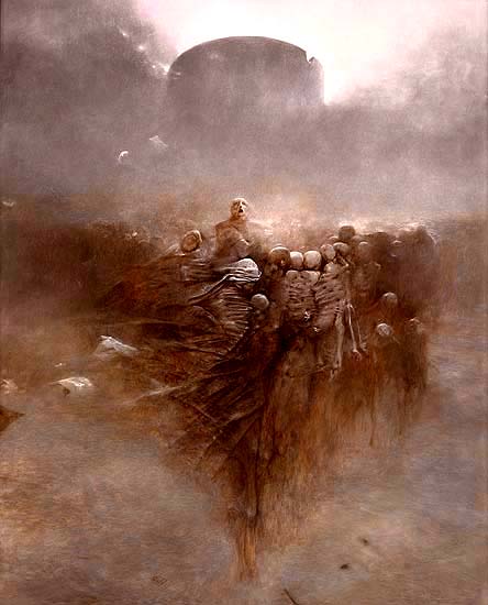

These are some paintings by
Zdzisław Beksiński.
April 2, 2022
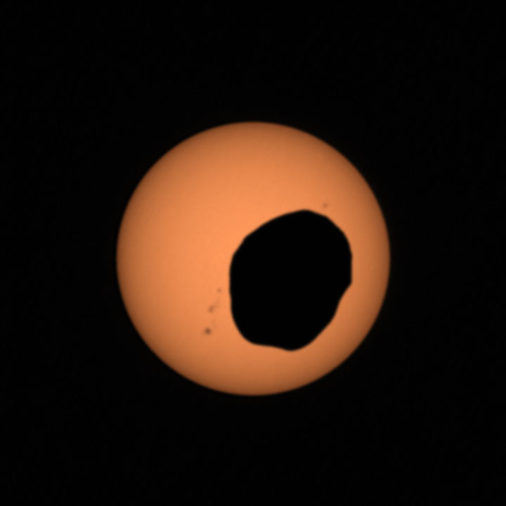
Solar eclipses on Mars look really different than they do here on Earth. And this one, created by the Martian moon Phobos, lasted just 40 seconds! Details here:
Above you see a 'standing wave', but the wave equation also has 'traveling wave' solutions:
The wave equation is 'linear', so we can add solutions and get new ones. In fact the standing wave I showed you is the sum of two traveling waves going in opposite directions:
In fact, every solution of the wave equation in 1d looks like this: $$ f(t,x) = g(x+t) + h(x-t) $$ \(g(x+t)\) is a wave moving to the left at speed 1. \(h(x-t)\) is a wave moving to the right at speed 1. Each of these waves can have any shape.
The wave equation in 2d space $$ \frac{\partial^2 f}{\partial t^2} - \frac{\partial^2 f}{\partial x^2} - \frac{\partial^2 f}{\partial y^2} = 0$$ has some solutions that are waves traveling in one direction, like this:
But you can get more interesting solutions by adding up waves going in lots of different directions! Here's a nice example:
It starts as a little 'wave packet'. It spreads out, since it's really a sum of waves going in different directions.
And just so you remember: the wave equation in 3 dimensions is $$ \frac{\partial^2 f}{\partial t^2} - \frac{\partial^2 f}{\partial x^2} - \frac{\partial^2 f}{\partial y^2} - \frac{\partial^2 f}{\partial z^2} = 0$$ or $$ \square f = 0 $$ for short.
But why am I telling you this? Because eventually I want to explain photons,
which are wave solutions of the vacuum Maxwell's equations!
April 9, 2022
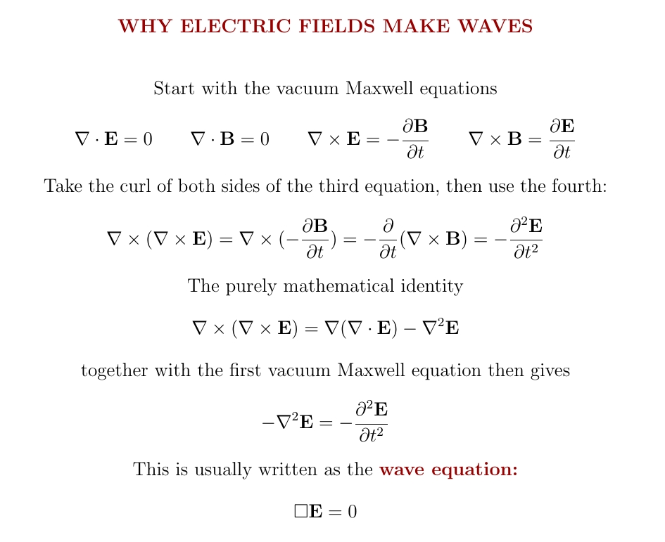
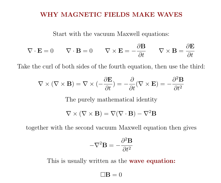
One of my favorite calculations: why electric fields make waves! We use the vacuum Maxwell equations and an identity involving the Laplacian $$ \nabla^2 = \frac{\partial^2}{\partial x^2} + \frac{\partial^2}{\partial y^2} + \frac{\partial^2}{\partial z^2} $$ which is part of the wave operator $$ \square = \frac{\partial^2}{\partial t^2} - \frac{\partial^2}{\partial x^2} - \frac{\partial^2}{\partial y^2} - \frac{\partial^2}{\partial z^2} $$ But the vacuum Maxwell equations have a symmetry between the electric and magnetic fields. So if the electric field obeys the wave equation, so must the magnetic field! We can see this directly by copying the argument that worked for the electric field.
But the vacuum Maxwell equations say more than just $$ \square \mathbf{E} = \square \mathbf{B} = 0 $$ For a wave moving in just one direction, called a 'plane wave', the electric and magnetic fields must point at right angles to each other... and to that direction!
You can see the proof of that fact here:
We say electromagnetic waves are 'transverse' because the fields point at right angles to the direction the wave is moving. People knew this before Maxwell, and spent a lot of time trying to explain it.Sound waves in air are 'longitudinal': the air vibrates along the direction the wave is moving, not at right angles to it. Sound in a solid can be either longitudinal or transverse.
So, back when scientists thought light was a vibration in a medium called 'aether', they struggled to understand why these vibrations are only transverse, never longitudinal. The aether would need to be an extremely rigid solid, because the speed of light is so high — and it would need to be completely incompressible, since there are no longitudinal waves of light!
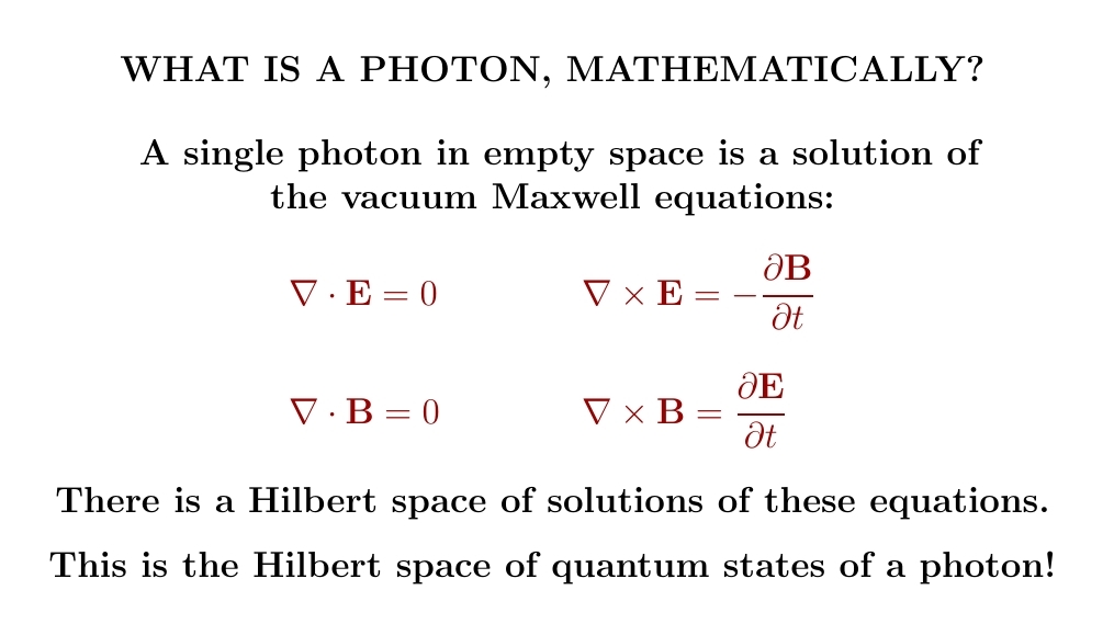
What is a photon? This is a complicated question. But a single photon in empty space has a simple description: it's a solution of the vacuum Maxwell equations.
Yes, solutions of the classical Maxwell equations also describe quantum states of a single photon!
But wait: quantum states are described by vectors in a complex Hilbert space. How do we multiply the quantum state of a photon by \(i\)?
If it has positive frequency, replace \(\mathbf{B}\) with \(\mathbf{E}\) and \(\mathbf{E}\) with \(-\mathbf{B}\). If it has negative frequency, replace \(\mathbf{B}\) with \(-\mathbf{E}\) and \(\mathbf{E}\) with \(\mathbf{B}\).
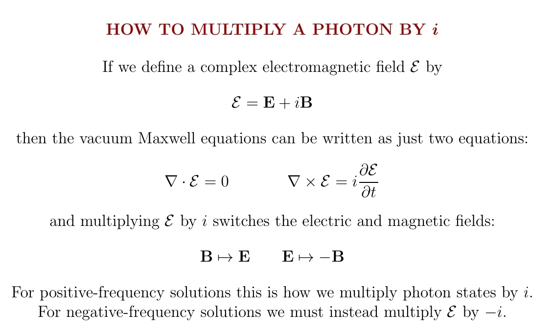
Why don't we just replace replace \(\mathbf{B}\) with \(\mathbf{E}\) and \(\mathbf{E}\) with \(-\mathbf{B}\) for both positive and negative frequency solutions of the vacuum Maxwell equations? Because then negative frequency solutions would work out to have negative energy! We don't want a theory with negative-energy photons.
To get a Hilbert space of photon states we also need to choose an
inner product for solutions of the vacuum Maxwell equations.
Up to scale, there's just one good way to do this that's invariant
under all the relevant symmetries. The formula is a bit scary:
$$ \langle (\mathbf{B},\mathbf{E}), (\mathbf{B}',\mathbf{E}') \rangle =
\int \!\int\! \int\! \left(\mathbf{B} \cdot \Delta^{-1/2} \,\mathbf{B}' +
\mathbf{E} \cdot \Delta^{-1/2}\, \mathbf{E}'\right) dx \,dy \,dz$$
Here we can define powers of the positive definite Laplacian \(\Delta
= - \nabla^2 \) using the Fourier transform.
April 15, 2022
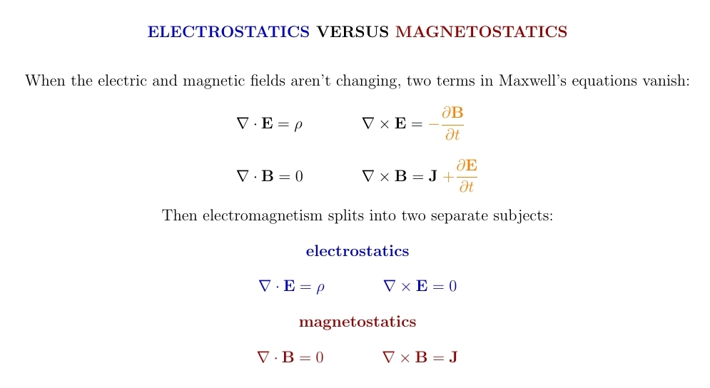
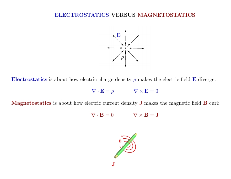
When the electric and magnetic fields change with time, they affect each other. But when they're unchanging, they don't! Then electromagnetism splits into two separate subjects, called electrostatics and magnetostatics.
The equations of electrostatics and magnetostatics look opposite from
each other. But tomorrow I'll show we can study them in similar ways,
using the electric 'scalar potential' and the magnetic 'vector
potential'. There will be hints of some deeper math.
April 16, 2022
Electrostatics is about how charge makes the electric field diverge —
without ever curling. Magnetostatics is about how current makes the
magnetic field curl — without ever diverging.
They're opposites. But there's a way to look at them that makes them very similar!
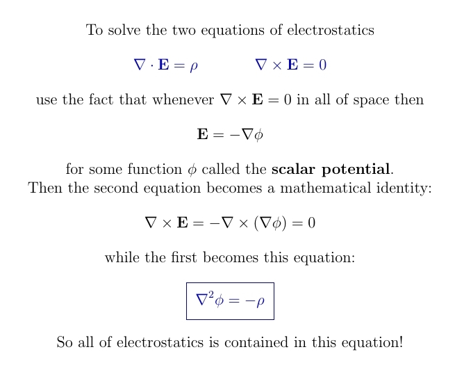
A great fact: a vector field on 3d Euclidean space has zero curl if and only if it's the gradient of some function.
So put in a minus sign just for fun and say the electric field is \(-\nabla \phi\) for some function \(\phi\) called the electric potential or scalar potential.
Then electrostatics boils down to just one equation!
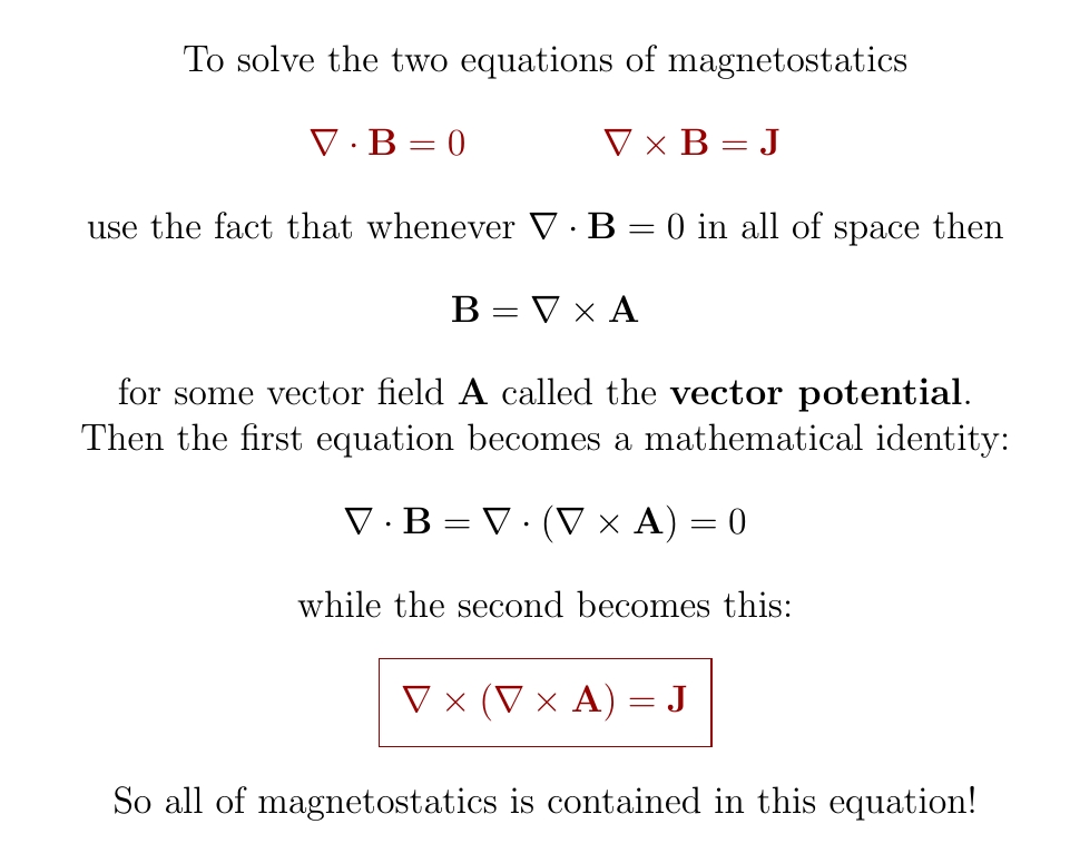
Another great fact: a vector field on 3d Euclidean space has zero divergence if and only if it's the curl of some vector field.
So say the magnetic field is \(\nabla \times \mathbf{A}\) for some vector field \(\mathbf{A}\).
Now magnetostatics also boils down to just one equation!
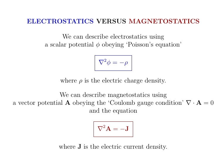
Yet another great fact: there are different choices of \(\mathbf{A}\) that have the same curl, and in 3d Euclidean space we can always pick a choice of \(\mathbf{A}\) with \(\nabla \times \mathbf{A} = \mathbf{B}\) whose divergence is zero.
So write \(\mathbf{B} = \nabla \times \mathbf{A}\) with \(\nabla \cdot \mathbf{A} = 0 \).
If we do this, magnetostatics looks a lot like electrostatics!

In short: electrostatics and magnetostatics look very similar if we use a scalar potential to describe the electric field and a vector potential for the magnetic field. This is the start of a deeper understanding of electromagnetism, called 'gauge theory'.
Also, the three "great facts" I used are part of an important branch of
math: De Rham
cohomology. It gets more interesting on spaces with holes.
Then these facts need to be adjusted to take the holes into account.
April 17, 2022
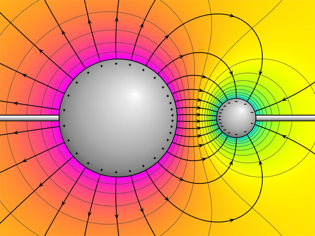
In electrostatics, the scalar potential \(\phi\) is pretty easy to visualize. The electric field points at right angles to the surfaces of constant \(\phi\), and it's stronger where these surfaces are more closely packed.
The nice picture here is by Geek3 on Wikicommons.
April 22, 2022
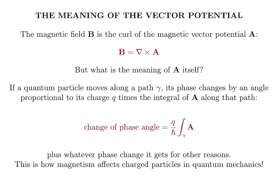
When you first meet the magnetic vector potential \(\mathbf{A}\) it's
mysterious. Its curl is the magnetic field. But what does it really
mean?
It helps to use quantum mechanics. Then \(\mathbf{A}\) is how a magnetic field affects the phase of a charged particle!
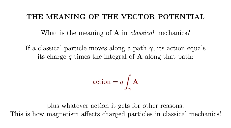
But we can also understand the vector potential \(\mathbf{A}\) using classical mechanics! When a classical charged particle moves along a path, its action is its charge times the integral of \(\mathbf{A}\) along that path...
...plus whatever action it gets for other, non-magnetic, reasons.
As a quantum particle moves along a path, its phase rotates. By what angle? By the action of the corresponding classical particle moving along that path, divided by Planck's constant \(h\). This was one of Feynman's greatest discoveries.
But you can only compare phase changes for two paths with the same starting point and ending point. So you can change \(\mathbf{A}\) in certain ways without changing anything physically observable. You can add the gradient of any function!
This is called gauge freedom.
Similarly, in classical mechanics you can only compare actions for two paths if they start at the same point and end at the same two point. But this 'gauge freedom' wasn't understood very well until quantum mechanics came along. So \(\mathbf{A}\) was mysterious.

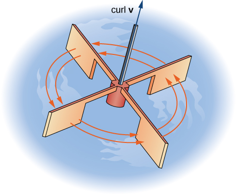
To understand the concept of 'curl', imagine water flowing with velocity vector field \(\mathbf{v}\). Imagine a tiny paddle-wheel with its center fixed at some point but free to rotate in all directions. Then it will turn with its axis of rotation pointing along the curl of \(\mathbf{v}\).
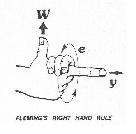
Alas, we need an arbitrary 'right-hand rule' or 'left-hand rule' to convert the wheel's rotation into a vector! We usually say the wheel rotates counterclockwise around the curl of \(\mathbf{v}\).
To avoid this arbitrary convention, we should use better math. Better math reveals that various things we'd been calling 'vectors' are not all the same. Using vectors to describe the curl is a hack! It uses an arbitrary rule... which changes into a different rule if we look at things in a mirror.
The full story is rather long, but when we write \(\mathbf{B} = \nabla \times \mathbf{A}\), the vector potential \(\mathbf{A}\) really points somewhere, while the magnetic field \(\mathbf{B}\) does not — it's a 'pseudovector'. Taking the curl again, the current density \(\mathbf{J} = \nabla \times \mathbf{B}\) really points somewhere!
You may be wondering why I haven't said your favorite word yet —
'differential form', or 'bivector', or whatever. These kinds of math
are very important because they're better at distinguishing different
kinds of vector-like things. But the full story is a bit bigger. In
3-dimensional space, each different 3d irreducible representation of
\(\mathrm{GL}(3, \mathbb{R})\) is a kind of vector-like thing. There
are lots of them — infinitely many, in fact. And a lot of them are
useful in physics. I'll talk about them tomorrow!
April 26, 2022
Vectors, polar vectors, axial vectors, pseudovectors, covectors,
bivectors and 2-forms. What are all these things? Some are just
synonyms, but there are a lot of different things like vectors in 3d
space.
Each of these different vector-like things forms a 3-dimensional representation of the group of \(3\times 3\) invertible real matrices. This group is called \(\mathrm{GL}(3,\mathbb{R})\). \(\mathrm{GL}\) stands for 'general linear group' the group of all linear coordinate transformations.
Even better, let's work in a coordinate-free way. Let \(V\) be any 3-dimensional real vector space. Let \(\mathrm{GL}(V)\) be the group of all invertible linear transformations of \(V\). \(V\) is a representation of \(\mathrm{GL}(V)\) in an obvious way.
Elements of \(V\) are 'vectors' in 3d space.
But \(\mathrm{GL}(V)\) has a lot of other 3-dimensional representations! For starters, let \(V^*\) be the dual vector space of \(V\): the space of all linear maps from \(V\) to \(\mathbb{R}\).
Elements of \(V*\) are called 'covectors', 'linear forms', or sometimes '1-forms'.
In classical mechanics, velocity is a vector while momentum is a covector. We can identify covectors with vectors using an inner product, but they transform differently under general linear coordinate transformations. So, we often distinguish between them.
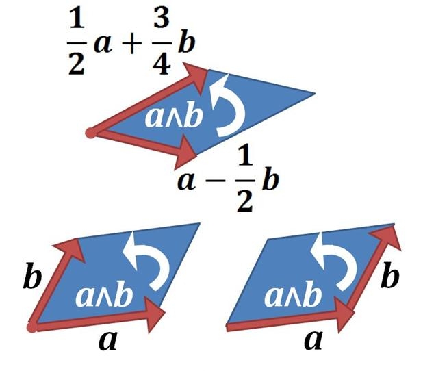
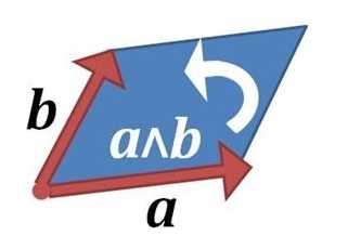
Next there's \(\Lambda^2(V)\), the second exterior power of \(V\). Elements of this are wedge products of two vectors, like \(a \wedge b\) here. You can draw them as oriented area elements. They are called 'bivectors'.
Details here:
We can identify bivectors with vectors using an inner product and an orientation on \(V\) - that's what's lurking in the 'right-hand rule'. But they are different as representations of \(\mathrm{GL}(V)\) .
If vectors have dimensions of length, bivectors have dimensions of length².
Next there's \(\Lambda^2(V^\ast)\), the second exterior power of the dual of V. Elements of this are often called '2-forms'. The use of a 2-form is that you can integrate it over an oriented surface and get a number.
In terms of units:
(In units where Planck's constant is 1, momentum has units of 1/length, because it's a covector.)
So far I've described four inequivalent 3-dimensional representations of \(\mathrm{GL}(V)\), or more concretely speaking \(\mathrm{GL}(3,\mathbb{R})\), all important in physics. All are irreducible representations.
But in fact, there are infinitely many 3d irreducible representations of \(\mathrm{GL}(3,\mathbb{R})\). They've all been classified.
For example there are 'pseudovectors', also known as 'axial vectors'. These are just vectors with a modified action of \(\mathrm{GL}(V)\).
To transform a pseudovector by \(g \in \mathrm{GL}(V)\), first let \(g\) act in the usual way on \(V\) and then multiply by
$$ \mathrm{det}(g)/|\mathrm{det}(g)| $$
which is \(\pm 1\).
When people call pseudovectors 'axial vector', they often call ordinary vectors 'polar vectors'.
To get all 3d irreducible representations of \(\mathrm{GL}(V)\), first let \(g \in (\mathrm{GL}(V)\) act as usual on either \(V\) or \(V^*\). Then 'densitize': multiply by \(|\mathrm{det}(g)|^p\) for some real number p. That gives half of them; for the rest also do the 'pseudo' trick and multiply by \(\mathrm{det}(g)/|\mathrm{det}(g)|\).
In physics 'densitizing' is a way to change the units of a quantity, multiplying it by some power of length. I mentioned that vectors have units of length. But if we densitize them as described, we get things with units of length\({}^{3p+1}\). We can make \(3p+1\) be be whatever we want. And not only can we densitize vectors and covectors, we can densitize tensors of any sort using the same trick:
As an exercise, figure out how to get the representation of \(\mathrm{GL}(V)\) on bivectors, \(\Lambda^2(V)\), using the tricks I just described.
I'll give you a hint: you have to start with \(V^\ast\). But then you have to
densitize by the right amount. And do you need to 'pseudoize'?
April 27, 2022
We can convert bivectors in 3d space into vectors, and vice versa, if we have an inner product and also an 'orientation' on that space: a choice of what counts as right-handed. But not all 3d vector spaces come born with this extra structure! So in general, vectors and bivectors are useful for different things.

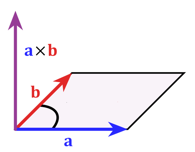
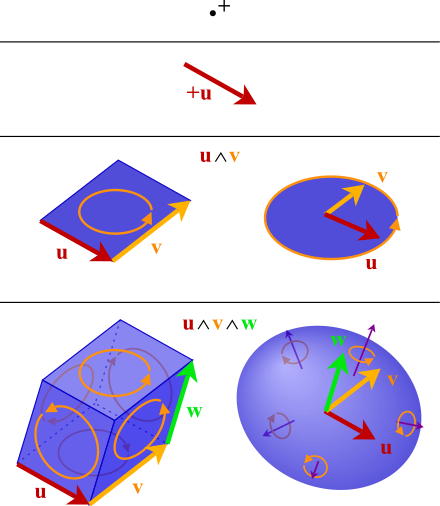
Similarly, you can multiply 3 vectors \(\mathbf{u},\mathbf{v},\mathbf{w}\) in a 3-dimensional vector space and get a trivector \(\mathbf{u} \wedge \mathbf{v} \wedge \mathbf{w}\), which looks like this purple thing. But if you have an inner product and orientation, you can convert that trivector into the number \(\mathbf{u} \cdot (\mathbf{v} \times \mathbf{w}\).
If you've only learned about the dot product and cross product, here's some good news: this is the start of a bigger, ultimately clearer story! Part of this story uses multivectors:
April 28, 2022
When I was a kid I was upset that Einstein never won a Nobel prize for
special or general relativity. I thought it was boring that he only
won a Nobel for the photoelectric effect. Later I realized this was
his most radical discovery — still mysterious to this day.
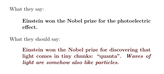
This isn't quite historically accurate. Einstein did make the remarkable leap toward realizing that light comes in quanta in his 1905 paper. Indeed, he wrote:
According to this picture, the energy of a light wave emitted from a point source is not spread continuously over ever larger volumes, but consists of a finite number of energy quanta that are spatially localized at points of space, move without dividing and are absorbed or generated only as a whole.
But in 1921 the Nobel committee only recognized him for his work on the photoelectric effect, not mentioning quanta. Only in 1922 did Compton come up with evidence that convinced everyone photons exist — and the name photon was introduced still later, in 1926, by the chemist Gilbert Lewis.
For more, see:
By the way, Planck really didn't understand the meaning of his own mathematics — it took Einstein to take quanta seriously. As Planck said in 1931, his introduction of energy quanta in 1900 was "a purely formal assumption and I really did not give it much thought except that no matter what the cost, I must bring about a positive result." For more on this, see:
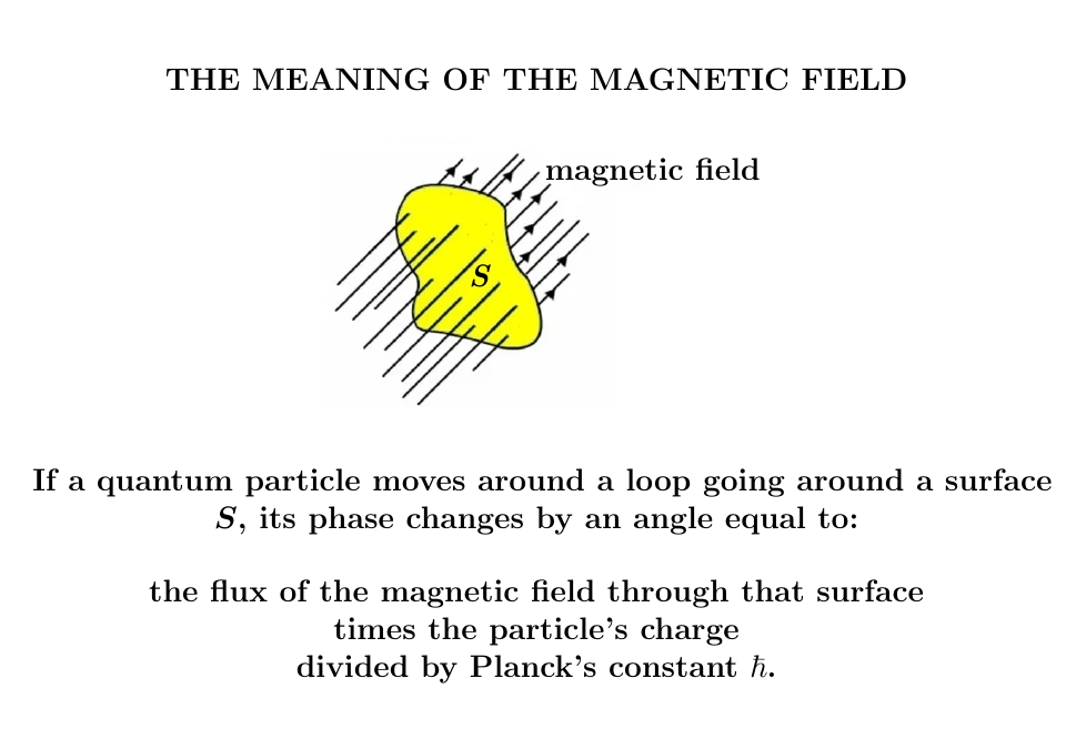
In quantum mechanics, the magnetic field says how much the phase of a charged particle rotates when you move that particle around a loop! (Not counting other effects.) This means that the magnetic field is fundamentally something you want to integrate over a surface.
So, while we often act like the magnetic field is a vector field, it's fundamentally a '2-form'. This is something you can integrate over an oriented surface. Converting a 2-form into a vector field forces you to use a 'right-hand rule'. And that's awkward.
You can integrate a 2-form over an oriented surface... but what is a 2-form, actually? It's linear map from bivectors to real numbers! A bivector is like a tiny piece of oriented area.
So how does the magnetic field eat a tiny piece of oriented area and give a number?
Here's how: if you move a charged particle around a tiny piece of
oriented area, its phase changes by some tiny angle. And that angle
is what the magnetic field tells you!
April 30, 2022
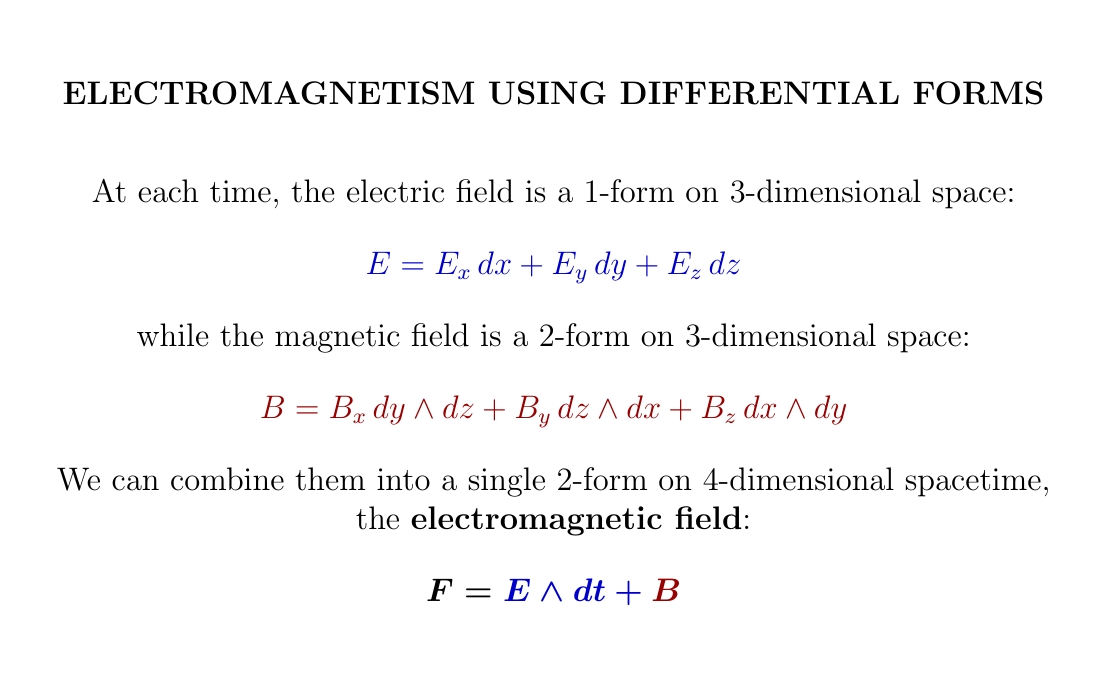
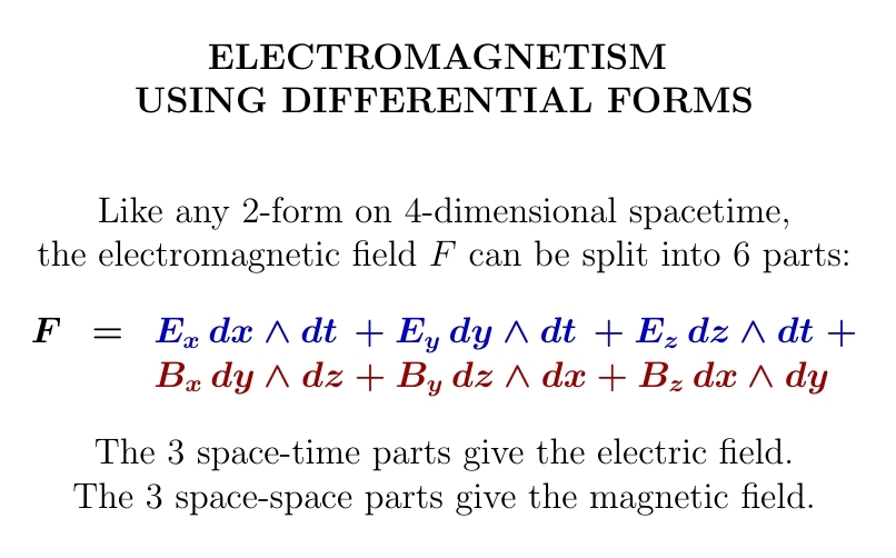
The electric and magnetic fields are very different when viewed as fields on space. But we can unify the electric and magnetic fields into a single field on spacetime: the electromagnetic field.
To do this, it helps to use 1-forms and 2-forms.
In quantum mechanics the magnetic field says how the phase of a charged particle changes when you move it around a little loop in the \(x,y\) directions, or the \(y,z\) directions, or \(z,x\).
The electric field does the same for the \(x,t\) directions, or \(y,t\) or \(z,t\).
There's a lot more to say about this! To explain electromagnetism clearly, I would need to introduce quantum mechanics, and differential forms, and now the spacetime perspective — so, special relativity. So the job keeps getting bigger.
Nature is a unified whole.