For my July 2020 diary, go here.

Diary — August 2020

John Baez

In this illusion by Akiyoshi Kitaoka the heart seems to shift, especially if you move your head a little.

August 2, 2020

I'm listening to lots of baroque music now. For some reason I listened to Albinoni's oboe concertos on YouTube:

I was blown away, because while I'd listened to tons of Bach and a tiny amount of Vivaldi (mainly the Four Seasons), I hadn't really listened to their contemporaries, or immediate predecessors.

I realize now it's crazy to listen to Bach and like him and not be able to know what's really him and what's just a common style of that time. It's like listening to just one jazz musician, or just one rock group. Imagine someone in the far future listening only to two 20th-century composers: Miles Davis and the Beatles. They would sound great, but all the context would be missing.

So I've been listening to Albinoni, and then I started listening to the complete works of Corelli, which are also on YouTube, and liked them so much I bought them: 10 CDs, a massive amount of music.

I used to listen to music in a sort of haphazard way, just whatever I bumped into that I liked best, but now that I'm getting old I feel a desire to get to know some musicians I like more 'completely'. And I'm excited that standing right behind the classical composers we all know about, starting roughly with Bach, there's this realm of baroque music that's really rich, just waiting to be explored!

August 4, 2020

A rotation in 4 dimensions is almost the same as a pair of rotations in 3 dimensions. This is a special fact about 3- and 4-dimensional space that doesn't generalize. It has big implications for physics and topology. Can we understand it intuitively?

Probably not, but let's try. For any rotation in 3d, you can find a line fixed by this rotation. The 2d plane at right angles to this line is mapped to itself. This line is unique except for the identity rotation (no rotation at all), which fixes every line.

For any rotation in 4d, you can find a 2d plane mapped to itself by this rotation. At right angles to this plane is another 2d plane, and this too is mapped to itself.

Each of these planes is rotated by some angle. The angles can be different. They can be anything.

A very special sort of rotation in 4d has both its 2d planes rotated by the same angle. Let me call these rotations 'self-dual'.

Another very special sort has its 2d planes rotated by opposite angles. Let me call these rotations 'anti-self-dual'.

(To tell the difference between self-dual and anti-self-dual rotations we need a convention, the 4d equivalent of a right-hand rule.)

Amazingly, self-dual rotations in 4 dimensions form a group! In other words: if you do one self-dual rotation and then another, the result is a self-dual rotation again. This is not obvious. Also, any self-dual rotation can be undone by doing some other self-dual rotation. That's pretty obvious.

Similarly, anti-self-dual rotations in 4 dimensions form a group. And this is isomorphic to the group of self-dual rotations.

What is this group like?

Another amazing fact: it's almost the group of rotations of three-dimensional space.

The group of self-dual (or anti-self-dual) rotations in 4d space is also known as \(\mathrm{SU}(2)\). This is not quite the same as the group of rotations in 3d space: it's a 'double cover'. That is, two elements of \(\mathrm{SU}(2)\) correspond to each rotation in 3d space.

If I were really good, I could take a self-dual rotation in 4d space, and see how it gives a rotation in 3d space. I could describe how this works, without using equations. And you could see why two Different self-dual rotations in 4d give the same rotation in 3d. But I haven't gotten there yet. So far, I only know how to show these things using equations. (They're very pretty if you use quaternions.)

Another amazing fact: you can get any rotation in 4d by doing first a self-dual rotation and then an anti-self-dual one.

And another amazing fact: self-dual rotations and anti-self-dual rotations commute. In other words, when you build an arbitrary rotation in 4d by doing a self-dual rotation and an anti-self-dual rotation, it doesn't matter which order you do them in.

All these amazing facts are all summarized in two equations. In 3d the group of rotations is called \(\mathrm{SO}(3)\). In 4d it's called \(\mathrm{SO}(4)\). The group \mathrm{SU}(2) has two special elements called \(\pm 1\). And we have $$ \mathrm{SO}(3) = \mathrm{SU}(2)/\pm 1 $$ $$ \mathrm{SO}(4) = (\mathrm{SU}(2)\times \mathrm{SU}(2)/\pm (1,1) $$ The first equation here says that \(\mathrm{SU}(2)\) is a double cover of the 3d rotation group: every element of \(\mathrm{SO}(3)\) comes from exactly two elements of \(\mathrm{SU}(2)\), and both \(1\) and \(-1\) in \(\mathrm{SU}(2)\) give the identity rotation (no rotation at all) in 3d.

The second equation here says that every rotation in 4d can be gotten by doing a self-dual rotation and an anti-self-dual rotation, each described by an element of \(\mathrm{SU}(2)\). It says the self-dual and anti-self-dual rotations commute. And it says a bit more! It also says that each rotation in 4d can be gotten in two ways by doing a self-dual rotation and an anti-self-dual rotation. Thus, \(\mathrm{SU}(2) \times \mathrm{SU}(2)\) is a double cover of \(\mathrm{SO}(4)\).

What I really want to do now is get better at visualizing this stuff and explaining it more clearly. Maybe you can help me out!

August 5, 2020

How did this happen?

The tweet became pretty popular, with almost 1000 likes, and it was retweeted by Eric Weinstein, a mathematician who I was friends with back when I taught at Wellesley College for two years. Weinstein is now the managing director of Thiel Capital. This is the investment firm of Peter Thiel, the head of PayPal.

Weinstein has a huge following on Twitter. He told me:

I think she just started following me today. So the follow may actually be from this tweet. Interesting if true.

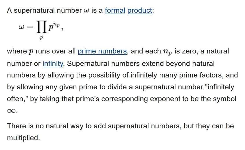
Wikipedia: "There is no natural way to add supernatural numbers."

Me: "Well duh. Try a supernatural way!"

Jens Hemelaer has a great blog article on supernatural numbers:

• Jens Hemelaer, Algebraic extensions and supernatural numbers, Tapis & Topos, August 6, 2020.

Supernatural numbers show up when you think about finite versus infinite-sized algebraic gadgets.

Suppose \(A\) is an \(2 \times 2\) matrix. Then there's a way to turn it into a \(6 \times 6\) matrix like this: $$ \left( \begin{array}{ccc} A & 0 & 0 \\ 0 & A & 0 \\ 0 & 0 & A \\ \end{array} \right) $$ where all the \(0\)s are really \(2 \times 2 \) blocks of zeros.

You can use the same type of trick to turn any \(n \times n\) matrix into an \(nm \times nm\) matrix. I just did the case \(n = 2, m = 3\).

This trick turns an \(n \times n\) matrix \(A\) into an \(nm \times nm\) matrix \(f(A)\) with copies of \(A\) down the diagonal and zeros elsewhere. Notice: $$ \begin{array}{rcl} f(A+B) &=& f(A)+f(B) \\ f(AB) &=& f(A) f(B) \\ f(cA) &=& c f(A) \\ f(0) &=& 0 \\ f(1) &=& 1 \end{array} $$ whenever \(c\) is any constant and \(A\) and \(B\) are matries, so we say \(f\) is an 'algebra homomorphism'.

For example we can turn \(2 \times 2\) matrices into \(6 \times 6\) matrices, and turn \(6 \times 6\) matrices into \(30 \times 30\) matrices, and turn \(30 \times 30\) matrices into \(210 \times 210\) matrices...

And now for the supernatural part: we can imagine going on forever, and getting infinite-sized matrices!

We have a way to think of \(2 \times 2\) matrices as a subset of the \(6 \times 6\) matrices, which we think of as a subset of the \(30 \times 30\) matrices, and so on... so we take the union and get infinite-sized matrices. (Mathematicians call this trick a 'colimit'.)

Even better, we have a consistent way to add and multiply these infinite-sized matrices, so they form an 'algebra'. It's consistent because the map \(f\) that lets us reinterpret an \(n \times n\) matrix \(A\) as an \(nm \times nm\) matrix matrix \(f(A)\) is an algebra homomorphism.

But our algebra of infinite-sized matrices depends on a lot of choices! I chose

but I could have done something else. It turns out that in the end our algebra depends on a supernatural number!

You see, I chose a sequence of whole numbers each of which divides the one before. So at each step I'm throwing in some extra prime factors. I chose $$ 2,\;\;2 \times 3=6,\;\; 2 \times 3 \times 5=30,\;\; 2 \times 3 \times 5 \times 7=210, \dots $$ but I could have done $$ 2 \times 2=4,\;\; 2 \times 2 \times 2 \times 5=40,\;\; 2 \times 2 \times 2 \times 2 \times 5=80, \dots $$ or many other things. All that matters for our infinite-sized algebra is how many times each prime shows up 'in the end', as we go on forever.

Each prime can show up any finite number of times... or it can show up infinitely many times. And that's what a supernatural number is all about! Recall the Wikipedia article:

Now let's make this stuff sound fancy. The infinite-sized matrix algebras we're getting can be 'completed' to give 'uniformly hyperfinite C*-algebras'. And James Glimm proved that uniformly hyperfinite C*-algebras are classified by supernatural numbers!

For details, try this:

• Uniformly hyperfinite algebras.

Supernatural numbers also classify algebraic extensions of the finite field with \(p\) elements, \(\mathbb{F}_p\), for the same sort of reason.

I think they also classify additive subgroups of the rational numbers containing the integers! See how it works?

August 8, 2020

We can play a game. I think of an integer. You ask me what it is mod 1, mod 2, mod 3, mod 4, and so on, and I tell you. You try to guess the integer.

Can you guess it?

Notice that at any finite stage of this game you can't be sure about the answer.

The reason is that \(n!\) equals \(0 \bmod 1\), and \(0 \bmod 2\), and \(0 \bmod 3\)... and so on up to \(0 \bmod n\). So if some number \(k\) is a legitimate guess based on my answers to your first \(n\) questions, so is \(k + n!\).

So, I can cheat and change the number I have in mind, without you noticing.

But some answers are just inconsistent. For example if I tell you my number equals \(1 \bmod 2\), I have to tell you it's either \(1\) or \(3 \bmod 4\). If I say it's \(0 \bmod 4\), you'll know I'm cheating!

A profinite integer is a way for me to play this game forever without you ever being sure I'm cheating.

Every integer gives a profinite integer, since I can just pick an integer and play the game honestly.

But there are also other profinite integers.

There are lots of ways for me to play this game indefinitely, changing my integer infinitely many times, without you ever being sure that I'm cheating. These are the other profinite integers.

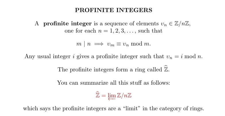
Profinite integers are very important in number theory. If \(\mathbb{F}_p\) is a finite field and \(\overline{\mathbb{F}_p}\) is its algebraic closure, then the Galois group of \(\overline{\mathbb{F}_p}\) over \(\mathbb{F}_p\) is the profinite integers! The reason is that \(\mathbb{F}_p\) has field extensions \(\mathbb{F}_{p^n}\) whose Galois groups are \(\mathbb{Z}/n\mathbb{Z}\), one for each \(n = 1, 2, 3, \dots\), and there's a way to take a union (or 'colimit', if you prefer) of these to get \(\overline{\mathbb{F}_p}\).

For more on profinite integers start here:

• Wikipedia, Profinite integer.

But you can teach profinite integers to kids by playing the game I described. If you keep cheating, they'll get it.

August 22, 2020

But this is probably not the explanation, since Descartes never actually used a coordinate grid, and never used negative numbers as coordinates — so he probably wasn't familiar with the four quadrants of modern Cartesian coordinates.

August 23, 2020

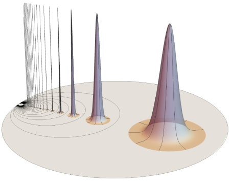
Jeremy Brazas studies 'wild topology'. So he looks at crazy spaces like this. We take a disk — think of it as the sea floor — and push it up to form an infinite sequence of hollow islands, all the same height, but ever narrower. It's called the 'harmonic archipelago'.

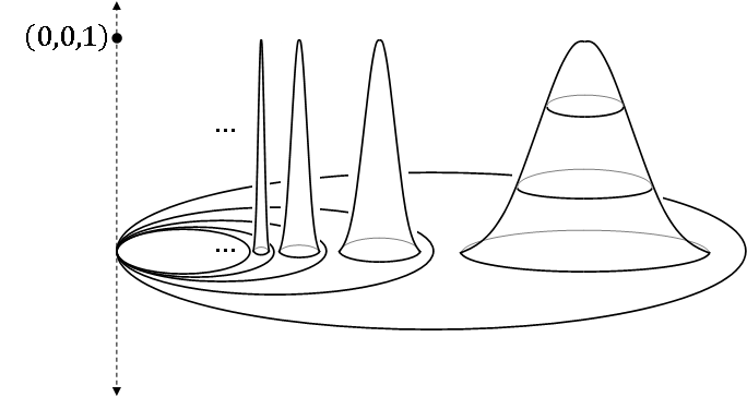
The first surprise is that the harmonic archipelago is not compact! The island peaks form a Cauchy sequence that does not converge, because the point (0,0,1) is not in this space.

But a bigger surprise comes when you try to compute its fundamental group. The fundamental group of the harmonic archipelago is uncountable!

Loops wrapping around infinitely many islands are not contractible. For example, the loop wrapping around the rim of the disk. Or the loop going around any one of the circles here:

But there are many more complicated noncontractible loops. You can go clockwise around the biggest circle, then counterclockise around the next one, etc., ad infinitum.

The fundamental group of the 'earring space', shown here, is also uncountable.

But the fundamental group of the harmonic archipelago also has no nontrivial homomorphism to the integers! This makes it different from the fundamental group of the Hawaiian earring, of which it's a quotient. For more on the harmonic archipelago and Hawaiian earring, start with this blog post by Jeremy Brazas and then read others:

• Jeremy Brazas, The harmonic archipelago, Wild Topology, May 1, 2014.

His blog is full of exotic delights: strange spaces that test your intuitions.

August 24, 2020

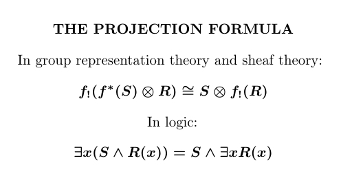
The 'projection formula' or 'Frobenius law' shows up in many branches of math, from logic to group representation theory to the study of sheaves. Let's see what it means in an example!

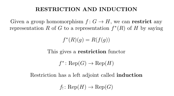
Given any group homomorphism \(f \colon G \to H\) you can 'restrict' representations of \(H\) along \(f\) and get representations of \(G\). But you can also take reps of \(G\) and freely turn them into reps of \(H\): this is 'induction'.

Induction is the left adjoint of restriction.

You can get a lot of stuff just knowing that induction is the left adjoint of restriction: this is called 'Frobenius reciprocity'.

But you can also take tensor products of representations, and then a new fact shows up: the projection formula!

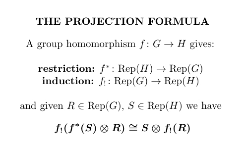
Where does this mysterious fact come from? It comes from the fact that the category of representations of a group is a symmetric monoidal closed category, and restriction preserves not only the tensor product of representations, but also the internal hom!

You get the projection formula whenever you have adjoint functors between symmetric monoidal closed categories and the right adjoint is symmetric monoidal and also preserves the internal hom! I wrote up a proof here:

• nLab, Frobenius reciprocity: closed monoidal functors and the projection formula.

This may not help you much unless you know some category theory and/or you've wrestled with the projection formula and wondered where it comes from. But to me it's a tremendous relief. I thank Todd Trimble for getting to the bottom of this and explaining it to me.

August 25, 2020

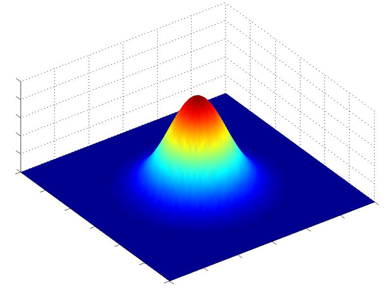
I have a Gaussian distribution like this in 2d. You know its variance is 1 but don't know its mean. I randomly pick a point \(\vec{x}\) in the plane according to this distribution, and I tell you what it is. You try to guess the mean of my distribution.

Your best guess is \(\vec{x}\).

That seems obvious — what could be better? But it's not true in 3 dimensions! This is called Stein's paradox, and it shocked the world of statistics in 1956.

But I need to state it precisely. An estimator is a function that provides a guess of the mean given the sample point \(\vec{x} \in \mathbb{R}^n\). We seek an estimator with smallest average squared error.

It's easy to create an estimator that does well sometimes. For example, suppose your estimator ignores the sample point and always guesses the mean is \(\vec{0}\). Then if the mean of my Gaussian actually is zero, you'll do great! But we want an estimator that does well always.

We say one estimator strictly dominates another if its average squared error is never bigger, regardless of the Gaussian's mean — and it's actually smaller for at least one choice of the Gaussian's mean.

Got it?

In 2d, no estimator strictly dominates the obvious one, where you guess the mean is the sample point \(\vec{x}\) that I've randomly chosen from my Gaussian distribution.

But in 3 or more dimensions, there are estimators that dominate the obvious one!!! Utterly shocking!!!

For example, in 3d you can take the sample point \(\vec{x}\), move towards the origin by a distance \(1/\|x\|\), and take that as your estimate of the mean. This estimator strictly dominates the obvious one where you guess \(\vec{x}\).

Insane! But the proof is here:

• Wikipedia, Proof of Stein's example.
• C. Stein, Inadmissibility of the usual estimator for the mean of a multivariate distribution, Proceedings of the Third Berkeley Symposium on Mathematical Statistics and Probability 1 (1956), 197–206.

In fact you don't need to move toward the origin. You could choose any point \(\vec{p}\) and always move the sample point \(\vec{x}\) towards that point by a distance \(1/\|\vec{x}-\vec{p}\|\). This estimator strictly dominates the obvious one.

So today my mind is a wreck. Common sense has been disproved, and I haven't yet found the new intuitions that make the truth seem reasonable to me. This is the life of a scientist. I've always sought this out. Things always make sense eventually.

One strange clue. Larry Brown showed that no estimator can strictly dominate the obvious one in \(n\) dimensions if and only if \(n\)-dimensional Brownian motion is 'recurrent' — that is, with probability one it comes back to where it was. This is true only for \(n \le 3\).

Larry Brown's argument is here:

• Larry D. Brown, Admissible estimators, recurrent diffusions, and insoluble boundary value problems, Ann. Math. Statist. 42 (1971), 855–903.

Here's a nice intro to Stein's paradox:

• Richard J. Samworth, Stein's paradox, Eureka 62 (2012), 38–41.

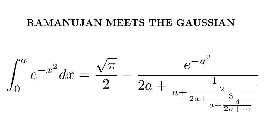
We all meet this integral in probability theory. Most of us don't respond as creatively as Ramanujan did! This was one of the formulas in his first letter to Hardy.

I just finished reading The Man Who Knew Infinity, Robert Kanigel's biography of Ramanujan. I recommend it to everyone. But I want to get a bit deeper into Ramanujan's math, so now I'm reading Hardy's book.

He said that Ramanujan's formula for the integral of the Gaussian "seemed vaguely familiar" when he first saw it, adding that "actually it is classical; it is a formula of Laplace first proved properly by Jacobi. Some other formulas in Ramanujan's letter were "much more intriguing", and a few were "on a different level and obviously both difficult and deep".

But I couldn't even begin to see why Ramanujan's formula for the Gaussian integral is true until I asked around.

August 27, 2020

$$ \Large{ \frac{4}{\pi} = 1 + \frac{1^2}{2 + \frac{3^2}{2 + \frac{5^2}{2 + \frac{7^2}{2 + \ddots}}}} } $$ Trying to understand a bit of Ramanujan's work, I realize I should start with the basics. This continued fraction expansion is one of many Euler discovered around 1748. They're not hard once you know the trick.

So let me tell you the trick!

You can turn sums into continued fractions using this formula: $$ a_0 + a_0a_1 + a_0a_1a_2 + \cdots + a_0a_1a_2\cdots a_n = $$ $$ \frac{a_0}{1 - \frac{a_1}{1 + a_1 - \frac{a_2}{1 + a_2 - \frac{\ddots}{\ddots \frac{a_{n-1}}{1 + a_{n-1} - \frac{a_n}{1 + a_n}}}}}} $$ It's called Euler's continued fraction formula. To convince yourself it's true, take the case n = 2. Simplify this fraction, starting from the very bottom and working your way up: $$ \frac{a_0}{1 - \frac{a_1}{1 + a_1 - \frac{a_2}{1 + a_2}}} $$ You'll get this: $$ a_0 + a_0a_1 + a_0a_1a_2 $$ And you'll see the pattern that makes the trick work for all \(n\).

To apply this trick, you need a series. Then write each term as a product. You may need to fiddle around a bit to get this to work. The arctangent function is a nice example. But try another yourself! $$ \begin{array}{ccl} \arctan x &=& \displaystyle{ \int_0^x \frac{d t}{1 + t^2} } \\ \\ & = & \displaystyle{ \int_0^x \left(1 - t^2 + t^4 - t^6 \cdots \right) dt } \\ \\ &=& \displaystyle{ x - \frac{x^3}{3} + \frac{x^5}{5} - \frac{x^7}{7} + \cdots } \\ \\ &=& x + x \left(\frac{-x^2}{3}\right) + x \left(\frac{-x^2}{3}\right)\left(\frac{-3x^2}{5}\right) + x \left(\frac{-x^2}{3}\right)\left(\frac{-3x^2}{5}\right)\left(\frac{-5x^2}{7}\right) + \cdots \end{array} $$ Now take your series and use Euler's continued fraction formula on it! You may get a mess at first. But you can simplify the fractions in it by multiplying the top and bottom by the same number: $$ \begin{array}{ccl} \arctan x &=& x + x \left(\frac{-x^2}{3}\right) + x \left(\frac{-x^2}{3}\right)\left(\frac{-3x^2}{5}\right) + x \left(\frac{-x^2}{3}\right)\left(\frac{-3x^2}{5}\right)\left(\frac{-5x^2}{7}\right) + \cdots \\ \\ &=& \Large{ \frac{x}{1 - \frac{\frac{-x^2}{3}}{1 + \frac{-x^2}{3} - \frac{\frac{-3x^2}{5}}{1 + \frac{-3x^2}{5} - \frac{\frac{-5x^2}{7}}{1 + \frac{-5x^2}{7} - \ddots}}}} } \\ \\ &=& \Large{ \frac{x}{1 + \frac{x^2}{3 - x^2 + \frac{(3x)^2}{5 - 3x^2 + \frac{(5x)^2}{7 - 5x^2 + \ddots}}}} } \end{array} $$ I'm optimistically assuming we can go on forever, but this is guaranteed to work whenever your original series converges.

So you've got a continued fraction formula for your function. Next, plug in some value of \(x\). You need \(x\) to be small enough for the series to converge.

Let's try \(x = 1\), since \(\arctan 1 = \pi/4\): $$ \frac{\pi}{4} = \frac{1}{1 + \frac{1^2}{3 - 1 + \frac{3^2}{5 - 3 + \frac{5^2}{7 - 5 + \ddots}}}} $$ Finally, simplify the formula to make it as beautiful as you can: $$ \frac{4}{\pi} = 1 + \frac{1^2}{2 + \frac{3^2}{2 + \frac{5^2}{2 + \frac{7^2}{2 + \ddots}}}} $$ Voilà!

You may enjoy this derivation of Euler's continued fraction formula, though it would be hard to do if you didn't know where you were heading:

• Wikipedia, Euler's continued fraction formula.

By the way, you can also see Euler's continued fraction formula as a generalization of the geometric series formula $$ a + a^2 + a^3 + \cdots = \frac{a}{1 - a} $$ to the case where we multiply each term in our series by a different number to get the next one, instead of multiplying by \(a\) each time.

August 30, 2020

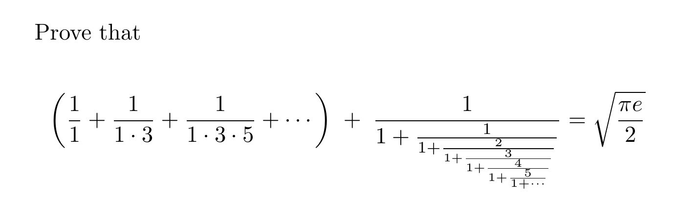
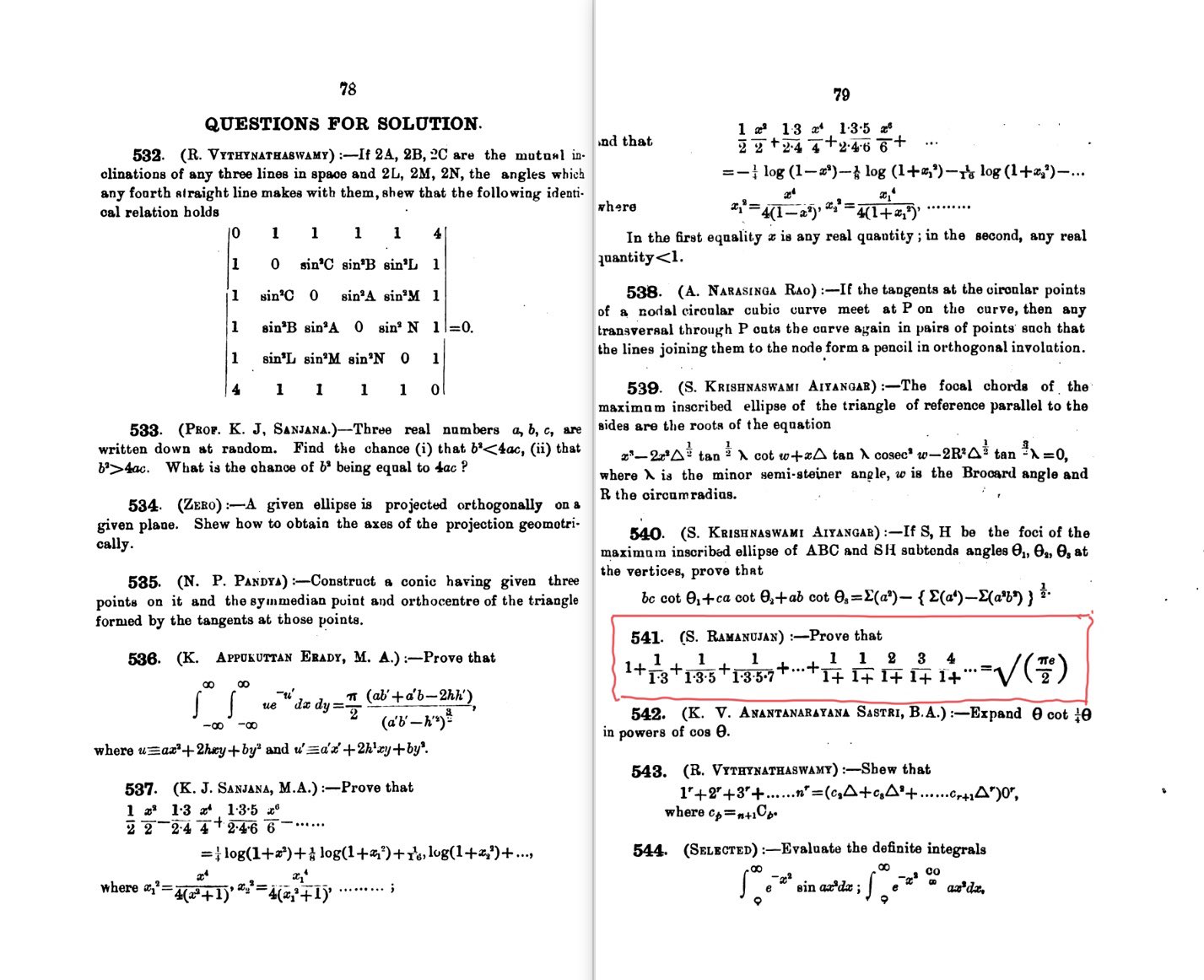
In 1914 Ramanujan posed this as Puzzle #541 in The Journal of Indian Mathematical Society. I decided it would be fun to try to understand this — using all the help I could get. You can see my first attempts here:

• John Baez, Chasing the Tail of the Gaussian (Part 1), The n-Category Café, August 31, 2020.

I've learned a lot about this puzzle-within-a-puzzle, but it's still mysterious to me. It goes back to Laplace's Traité de Mécanique Céleste — where he's calculating the refraction due to the Earth's atmosphere! But Laplace just writes down the formula without much explanation.

Here's one discussion of the issue:

• A continued fraction for error function by Ramanujan, Paramanand's Math Notes, June 21, 2014.

He studies some polynomials \(P_n, Q_n\) and claims that \(Q_n/P_n\) is the \(n\)th convergent of the continued fraction $$ \Large{ \frac{1}{1 + \frac{1}{1 + \frac{2}{x + \frac{3}{x + \frac{4}{x + \ddots}}}}} } $$ I don't see why this is true. I'm probably just being dumb. But after a while, I realized there's a much faster way to get ahold of the continued fraction — see below.

Here is the page where Ramanujan's puzzle first appeared - it's page 79 of Volume 6, Number 2 of The Journal of the Indian Mathematical Society which came out in April 1914. Amitabha Sen kindly provided a copy:

August 31, 2020

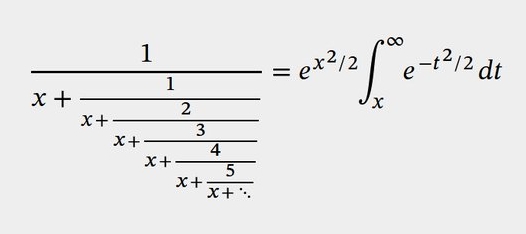
I finally solved this puzzle by Ramanujan!

But to compute the continued fraction, I broke down and "cheated" by reading a paper by Jacobi written in 1834 — in Latin. It was full of mistakes, but also brilliant. I explained it, and then my Twitter friend Leo Stein found a way to do Jacobi's calculation much more efficiently, which made me entirely rewrite my blog article:

• John Baez, Chasing the Tail of the Gaussian (Part 2), The n-Category Café, September 3, 2020.

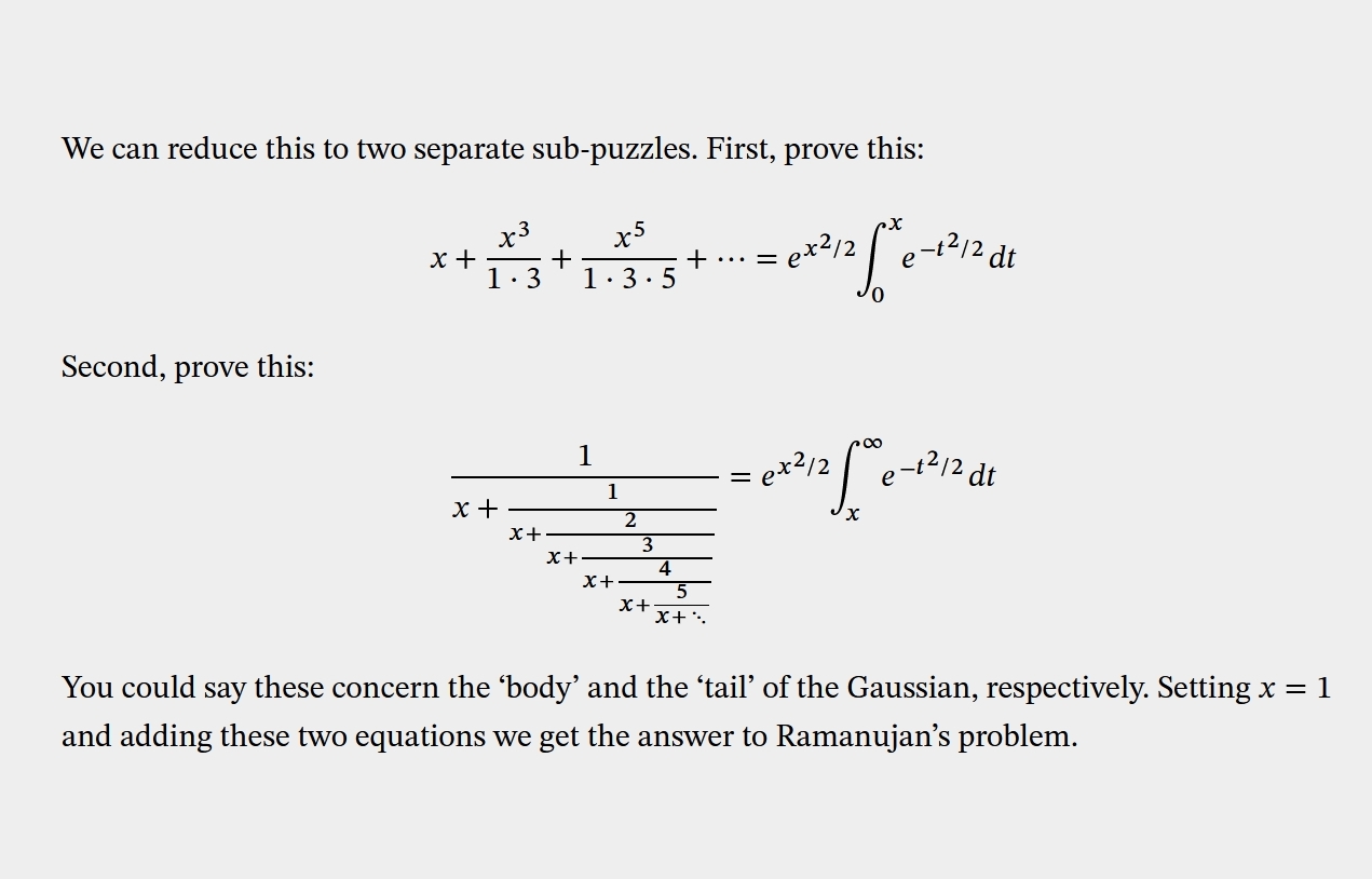
The cool part is that Ramanujan cleverly hid two puzzles in one! It seems you need to compute the infinite series and the continued fraction separately. The first involves the integral of a Gaussian from \(0\) to \(x\). The second involves the integral from \(x\) to \(\infty\). When you set \(x = 1\) and add them up you get \(\sqrt{\frac{\pi e}{2}}\).

To do the first sub-puzzle it helps to know how power series solve differential equations. I know that.

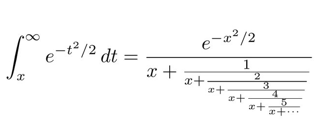
To do the second one you it helps to know how continued fractions solve differential equations. I didn't know that! That's where I needed help from Jacobi:

Jacobi's method is utterly magical! He shows the function at right here, say \(g(x)\), obeys a differential equation. He uses this to compute \(g\) in terms of \(g'/g''\), then \(g'/g''\) in terms of \(g''/g'''\), and so on forever until he gets the formula at left!

For my September 2020 diary, go here.

home