
In this wonderful illusion by Akiyoshi Kitaoka the black
hole appears to expand, though it does not.
July 2, 2020
I just learned a shocking theorem!
A bounded operator \(N\) on a Hilbert space is normal iff \(NN^* = N^*N\). Putnam's theorem says that if \(M\) and \(N\) are normal and $$ MT = TN $$ for some bounded operator \(T\), then $$ M^*T = TN^* $$ It's shocking because it's all just equations but you can't prove it just by fiddling around with equations. Rosenblum gave a nice proof. First note that \(MT = TN\) implies $$ M^n T = T N^n $$ for all \(n\). Then use power series to show $$ e^{cM} T = T e^{cN} $$ for all complex \(c\), so $$ \qquad \qquad \quad e^{cM} T e^{-cN} = T \qquad \qquad (\dagger) $$
Then the magic starts. Let $$ F(z) = e^{zM^*} T e^{-zN^*} $$ for complex \(z\). If we can show this is constant we're done, since differentiating with respect to \(z\) and setting \(z = 0\) gives $$ M^*T - TN^* = 0 $$ which shows \(M^*T = TN^*\).
But how can we show it's constant?
Well, 'obviously' we use Liouville's theorem: a bounded analytic function is constant. This is true even for analytic functions taking values in the space of bounded linear operators!
Now $$ F(z) = e^{zM^*} T e^{-zN^*} $$ is clearly analytic — but why is it bounded as a function of \(z\)?
We fiendishly note that $$ \begin{array}{ccl} F(z) &=& e^{zM^*} T e^{-zN^*} \\ &=& e^{zM^*} e^{-z^*M} T e^{z^*N} e^{-zN^*} \end{array} $$ since \(e^{-z^*M} T e^{z^*N} = T\) by \((\dagger)\). We then get $$ F(z) = e^{zM - (zM)^*} T e^{z^*N - (z^*N)^*} $$ since \(M\) commutes with \(M^*\) and \(N\) commutes with \(N^*\).
But \(zM - (zM)^*\) and \(z^*N - (z^*N)^*\) are skew-adjoint: that is, minus their own adjoint. So when you exponentiate them you get unitary operators, which have norm 1! So $$ \|F(z)\| \le \|T\| $$ so \(F(z)\) is bounded analytic and we're done.

Why this group? Can we derive it from beautiful math?
Yes! But I don't know if it helps.
First, the true symmetry group is not \(\mathrm{SU}(3)\times \mathrm{SU}(2)\times \mathrm{U}(1)\), it's \(\mathrm{S}(\mathrm{U}(3)\times \mathrm{U}(2))\): the group of \(5\times 5\) unitary matrices with determinant \(1\) that are block diagonal with a \(3\times 3\) block and a \(2\times 2\) block.
This group is \(\mathrm{SU}(3)\times \mathrm{SU}(2)\times U(1)\) mod a certain \(\mathbb{Z}_6\) subgroup, and it explains why quarks have charges \(2/3\) and \(-1/3\). For details, try Section 5 here:
So how can we get \(\mathrm{S}(\mathrm{U}(3)\times \mathrm{U}(2))\) to fall out of beautiful pure math?
Take the Jordan algebra of \(3\times 3\) self-adjoint octonionic matrices. Take the group of automorphisms that preserve a copy of the \(2\times 2\) self-adjoint complex matrices sitting inside it. It's \(\mathrm{S}(\mathrm{U}(3)\times \mathrm{U}(2))\).
This is intriguing because we know the Jordan algebras that can describe observables in finite quantum systems. They come in 4 infinite families, the most famous being the \(n\times n\) self-adjoint complex matrices.
Then there's one exception: \(3\times 3\) self-adjoint octonionic matrices! This is called the 'exceptional Jordan algebra'.
The \(2\times 2\) self-adjoint complex matrices are observables for a 'qubit'. They sit inside the \(3 \times 3\) self-adjoint octonionic matrices in many ways. The symmetries of this larger Jordan algebra that map the smaller one to itself are the symmetries of the Standard Model!
This was discovered by Michel Dubois-Violette and Ivan Todorov in 2018, and I explained it here:
Here's a new paper that tries to go further:
It's not the answer to all our questions... but I'm glad to see someone gnawing on this bone.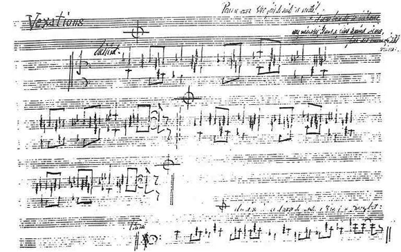
This is a fun article:
Though Erik Satie’s "Vexations" (1893) consisted of only a half sheet of notation, its recital had previously been deemed impossible, as the French composer had suggested at the top of his original manuscript that the motif be repeated eight hundred and forty times.Igor Levit did a live-streamed performance of "Vexations"; a small portion is here:Even before repetition, the piano line is unnerving: mild but menacing, exquisite but skewed, modest but exacting. Above the music, Satie included an author's note, as much a warning as direction: “It would be advisable to prepare oneself beforehand...."
The American composer John Cage was the first to insist that staging "Vexations" was not only possible but essential. No one knew what exactly would occur, which is part of what enticed Cage, who had a lust for unknown outcomes.
The performance commenced at 6 P.M. that Monday and continued to the following day’s lunch hour. To complete the full eight hundred and forty repetitions of "Vexations" took eighteen hours and forty minutes.
The New York Times sent its own relay team of critics to cover the event in its entirety... In the aftermath, some onlookers were bemused; others were agitated. Cage was elated. "I had changed and the world had changed," he later said.
In the years that followed its début, "Vexations" outgrew its status as a curiosity. It became a rite of passage. As performances flourished, its legend intensified... Recitals were part endurance trial, part vision quest.
Even after hundreds of repetitions, players are forced to sight-read from the beginning, as if learning for the first time. Witnesses have reported a similar effect. Listeners that subject themselves to the unnerving melody for several hours still find themselves incapable of humming it.
Those who sit for all eight hundred and forty repetitions tend to agree on a common sequence of reactive stages: fascination morphs into agitation, which gradually morphs into all-encompassing agony. But listeners who withstand that phase enter a state of deep tranquility.
An Australian pianist named Peter Evans abandoned a 1970 solo performance after five hundred and ninety-five repetitions because he claimed he was being overtaken by evil thoughts and noticed strange creatures emerging from the sheet music.
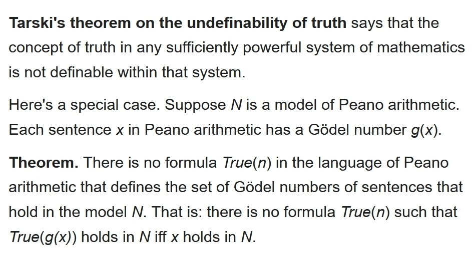
Roughly speaking, Tarski proved that truth within a system of math can't be defined within that system. Why not? If it could, you could create a statement in that system that means "this statement isn't true".
But there are some loopholes you should know about.
For one, you can define truth within some system of math using a more powerful system. Tarski actually constructed an infinite hierarchy of systems, each more powerful than the ones before, where truth in each system could be defined in all the more powerful ones!
But you can also do this: within Peano arithmetic, you can define truth for sentences that have at most \(n\) quantifiers!
Sorta like: "Nobody can give you all the money you might ask for, but for any \(n\) someone can give you up to \(n\) dollars."
This shocked me at first. Michael Weiss explained it to me on his blog.
Skip down to where I say "let me think about this a while as I catch my breath."
The reason there's no paradox is that when you try to build the sentence that says "this sentence is false", it has one more quantifier. But Michael explains how you can define truth for sentences with at most \(n\) quantifiers. It's an inductive construction, based on ideas of Tarski's. For more on his ideas, go here:
I think the moral is that while you can define mathematical truth
in stages, you can never finish.
July 11, 2020
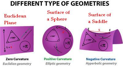
A 'Riemannian manifold' is, roughly speaking, a space in which we can measure lengths and angles. The most symmetrical of these are called 'symmetric spaces'. In 2 dimensions there are 3 kinds, but in higher dimensions there are more.
An 'isometry' of a Riemannian manifold \(M\) is a one-one and onto function \(f \colon M \to M\) that preserves distances (and thus, it turns out, angles). Isometries form a group. You should think of this as the group of symmetries of \(M\).
For \(M\) to be very symmetrical, we want this group to be big.
The group of isometries of a Riemannian manifold is a manifold in its own right! So it has a dimension.
For example the isometry group of the plane, sphere or hyperbolic plane is 3-dimensional. This is biggest possible for the isometry group of a 2d Riemannian manifold!
For an \(n\)-dimensional Riemannian manifold, how big can the dimension of its isometry group be? It turns out the maximum is \(n(n+1)/2\). And this happens in just 3 cases:
Another great bunch of examples come from 'Lie groups': manifolds that are also groups, such that multiplication is a smooth map.
The best Lie groups are the 'compact' ones. These can be made into Riemannian manifolds in such a way that both left and right multiplication by any element is an isometry!
We can completely classify compact Lie groups, and study them endlessly.
So, any decent definition of 'symmetric space' should include Euclidean spaces, spheres, hyperbolic spaces and compact Lie groups — like the rotation groups \(\mathrm{SO}(n)\), or the unitary groups \(\mathrm{U}(n)\). And there's a very nice definition that includes all these — and more!
A Riemannian manifold M is a symmetric space if it's connected and for each point \(x\) there's an isometry \(f \colon M \to M\) called "reflection through \(x\)" that maps \(x\) to itself and reverses the direction of any tangent vector at \(x\): $$ f(x) = x $$ and $$ df_x = -1 $$ For example, take Euclidean space. For any point \(x\), reflection through \(x\) maps each point \(x + v\) to \(x - v\). So it maps \(x\) to itself, and reverses directions!
To understand symmetric spaces better, it's good to draw or mentally visualize 'reflection around \(x\)' for a sphere.
We can completely classify compact symmetric spaces — and spend the rest of our lives happily studying them. Besides the compact Lie groups, there are 7 infinite families and 12 exceptions, which are all connected to the octonions:
(Some fine print is required for a complete match of definitions.)
Symmetric space are also great if you like algebra! Just as Lie groups can be studied using Lie algebras, symmetric spaces can be studied using '\(\mathbb{Z}/2\)-graded Lie algebras', or equivalently 'Lie triple systems'. I explained that approach here on June 24th.
Even better, the \(7+3 = 10\) infinite series of compact symmetric spaces (the seven I mentioned plus the three infinite series of compact Lie groups) are fundamental in condensed matter physics! They appear in the something called the '10-fold way', which classifies states of matter:
So, our search for the most symmetrical spaces leads us to a meeting-ground of algebra and geometry that generalizes the theory of Lie groups and Lie algebras and has surprising applications to physics! What more could you want?
Oh yeah, you might want to learn this stuff.
Wikipedia is good if you have the math background for it:
Finally, to really sink into the glorious details of symmetric spaces,
I recommend Arthur Besse's Einstein Manifolds. Besse is a
relative of the famous Nicolas Bourbaki. His book has lots of great
tables. It's lots of fun to browse!
July 12, 2020
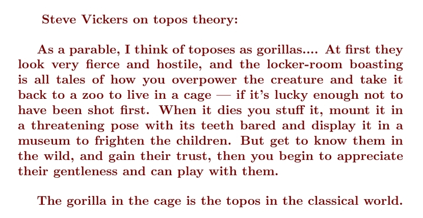
A topos is a universe in which you can do mathematics, with its own
internal logic, which may differ from classical logic.
On the category theory mailing list, Vaughan Pratt once doubted that anyone could really think using this internal logic, calling this locker-room boasting.
Steve Vickers replied as follows:
Here's my very quick intro to topos theory:
Here's the full exchange between Pratt and Vickers, which adds useful detail:
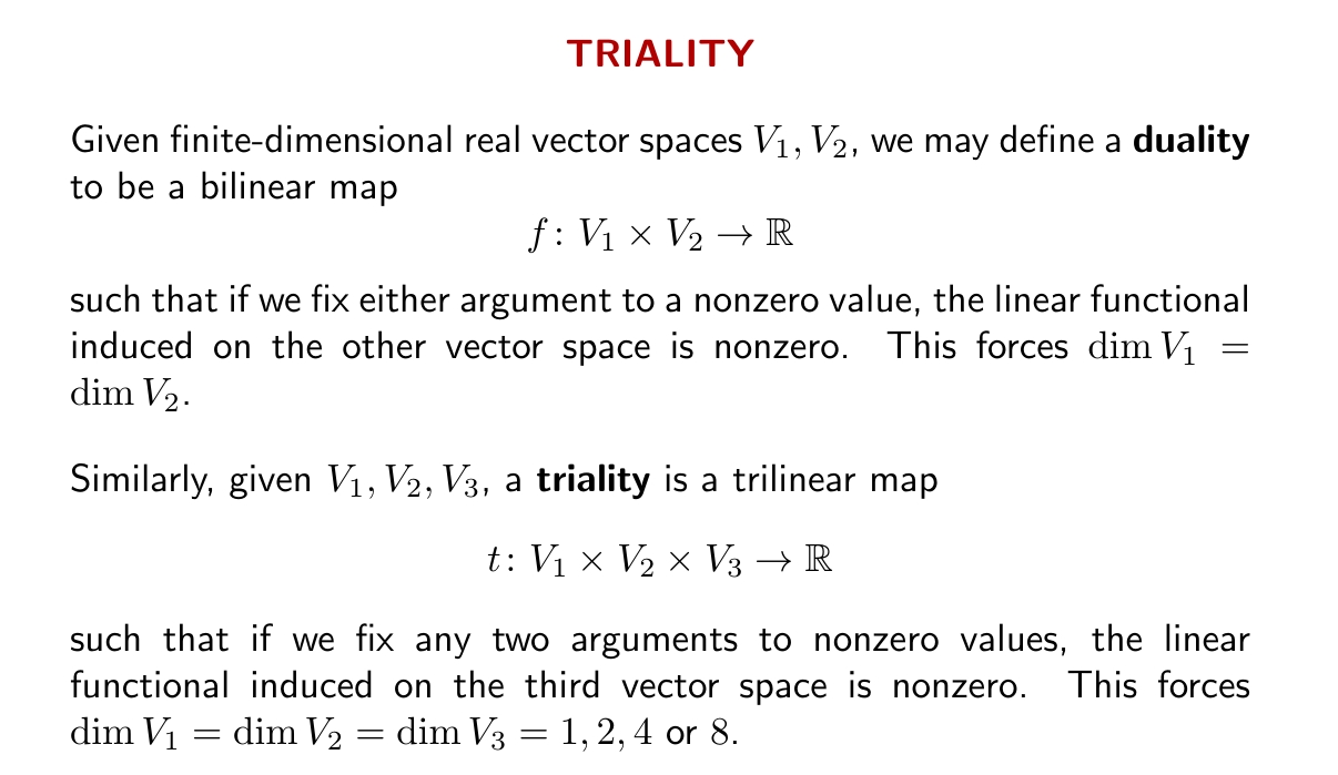
For example, take all three vector spaces to be \(\mathbb{C}\), the complex numbers, and define \(t(v_1,v_2,v_3) = \mathrm{Re}(v_1v_2v_3)\). This is a triality!
The same trick works if we start with the real numbers, the quaternions, or the octonions.
But wait! The octonions aren't associative! So what do I mean by \(\mathrm{Re}(v_1v_2v_3)\) then? Well, luckily $$ \mathrm{Re}((v_1v_2)v_3) = \mathrm{Re}(v_1(v_2v_3)) $$ even when \(v_1, v_2, v_3\) are octonions. The proof that finite-dimensional trialities can happen only in dimensions 1,2,4 or 8 is quite deep. It's easy to show any triality gives a 'division algebra', and I explain that here:
But then we need to use a hard topological theorem! It's pretty easy to show that if there's an \(n\)-dimensional division algebra, the \((n-1)\)-sphere is 'parallelizable': we can find \(n-1\) continuous vector fields on this sphere that are linearly independent at each point.In 1958, Kervaire, Milnor and Bott showed this only happens when \(n\) = 1, 2, 4, or 8.
So, trialities are rare. But once you have one, you can do lots of stuff.
Even better, the 'magic square' lets you take two trialities and build a Lie algebra. If you take them both to be the octonions, you get \(\mathrm{E}_8\).
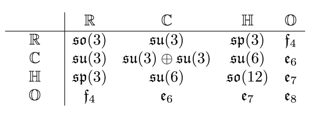
Details here:
And what's better than two trialities? Well, duh — three!!!Starting from three trialities — but not just any three — you can build a theory of supergravity. This gives the 'magic pyramid of supergravities':
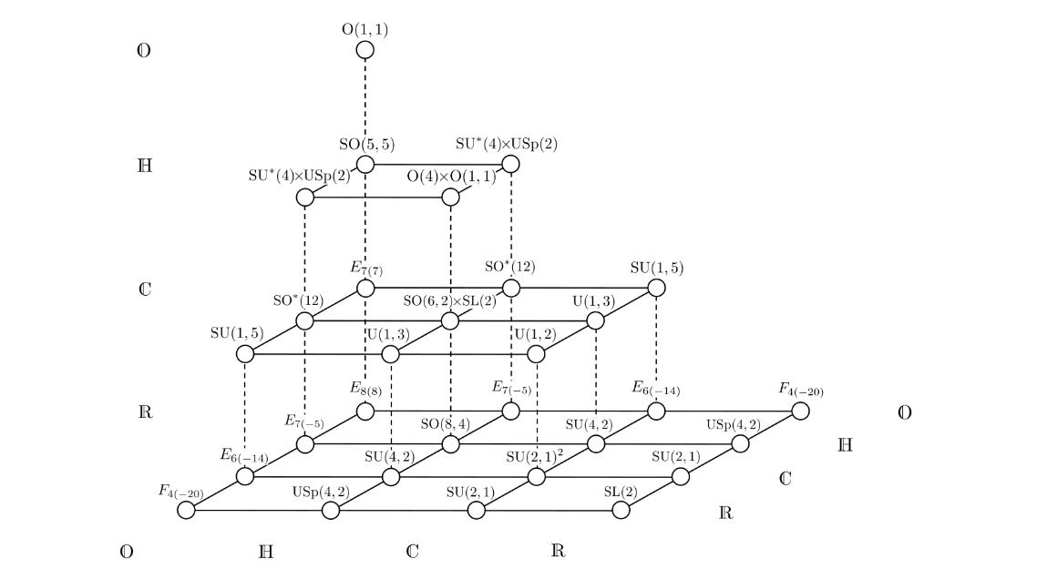
For more, read this:
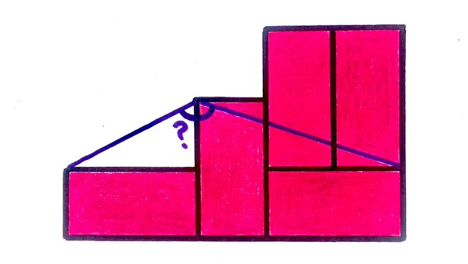
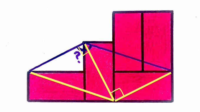
We can solve this in two ways. First, the rectangles must be twice as long as they are wide, so if we chop the mystery angle into two parts as below, we see it's $$ \arctan 2 + \arctan 3. $$

But Vincent Pantaloni chopped the mystery angle into two parts a different way, which makes it clear the angle is $$ \frac{\pi}{2} + \frac{\pi}{4} = \frac{3\pi}{4}. $$
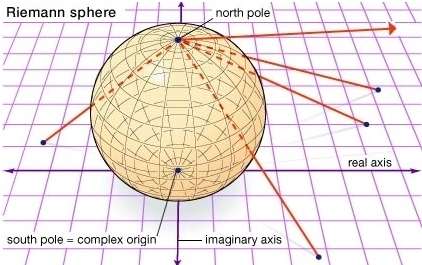
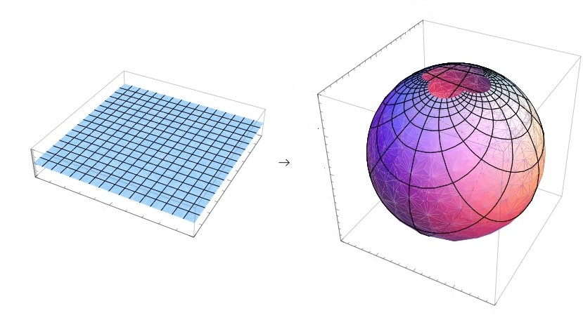
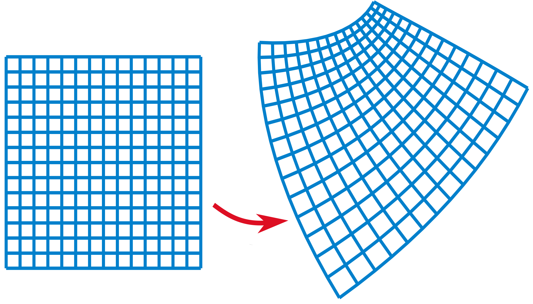
Take a sphere and set it on the plane. You can match up almost every point on the sphere with one on the plane, by drawing lines through the north pole.
There's just one exception: the north pole itself! So, the sphere is like a plane with one extra point added.
The interesting thing about this trick is that angles on the plane equal angles on the sphere!
So if you use this trick to draw a map of the Earth, distances get messed up but angles are preserved at each point. Antarctica would stretch on forever:
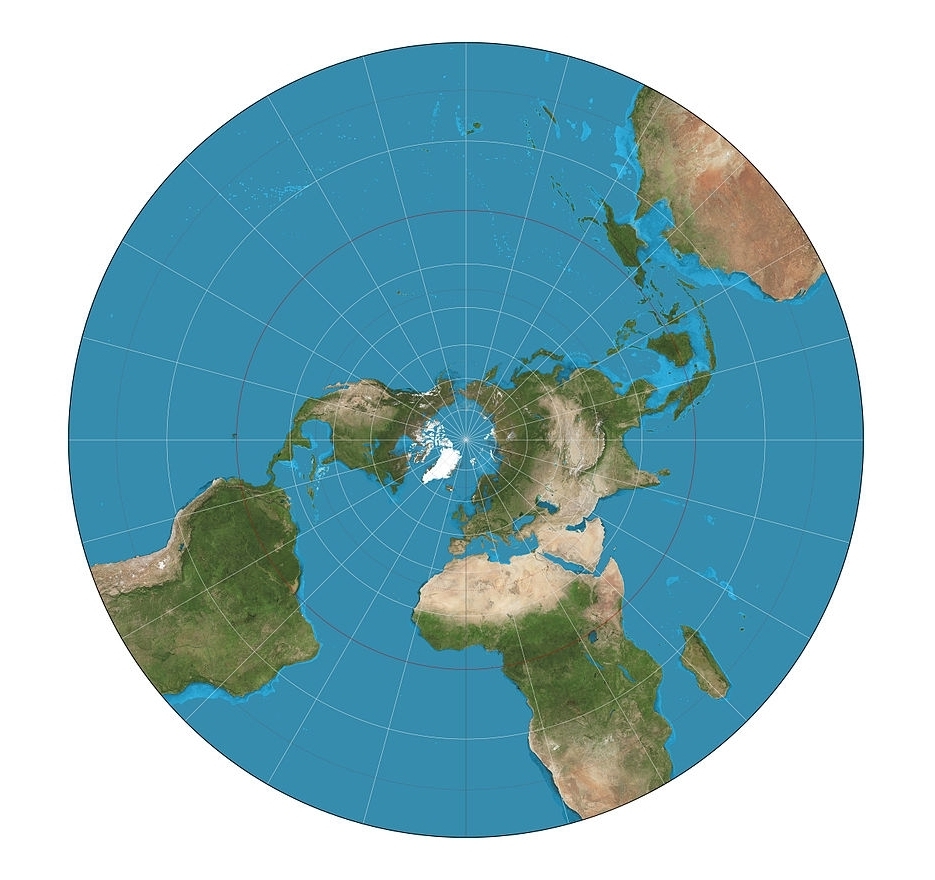
Some useful jargon: an angle-preserving mapping is called 'conformal'.
Mathematicians often call the plane 'the complex numbers', where a point \((x,y)\) is written as the number \(x+iy\). Then the sphere is called the 'Riemann sphere': the complex numbers plus one extra point, called \(\infty\). It lets us think of infinity as a number!
And here's a wonderful thing: any differentiable function from the complex numbers to the complex numbers preserves angles — except where its derivative is zero. So it's a conformal mapping!
The Riemann sphere is not some abstract thing, either. It's the sky! More precisely, if you're in outer space and can look in every direction, the 'celestial sphere' you see is the Riemann sphere.
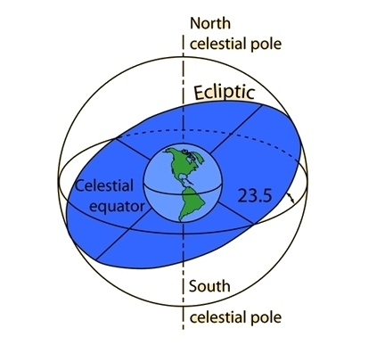
Now suppose you're moving near the speed of light. Thanks to special relativity effects, the constellations will look warped. But all the angles will be the same. Your view will be changed by a conformal transformation of the Riemann sphere!
A math book may summarize all this as follows: $$ \mathrm{SO}_0(3,1) \cong \mathrm{PSL}(2,\mathbb{C}). $$ In other words: the group of Lorentz transformations is isomorphic to the group of conformal transformations of the Riemann sphere!
So: when reading math, it's often your job to bring it to life.
July 18, 2020
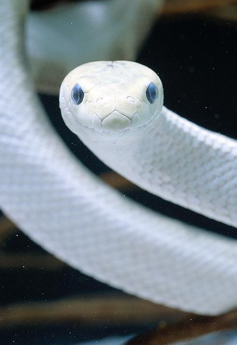
There's a lot of depressing news these days. Pictures of animals help
me stay happy. Here are some of my faves.
First: an insanely cute Cuban flower bat, Phyllonycteris
poeyi, photographed by Merlin Tuttle.

Second: a devilishly handsome Dracula parrot, Psittrichas fulgidus, photographed by Ondrej Prosicky. It lives in New Guinea. It subsists almost entirely on figs. It's also called Pesquet's parrot.

Third: the aptly named 'elegant sea snake', Hydrophis elegans.
It's elegant, but it's poisonous.
Fourth, a kitten of a Canada lynx, Lynx canadensis.

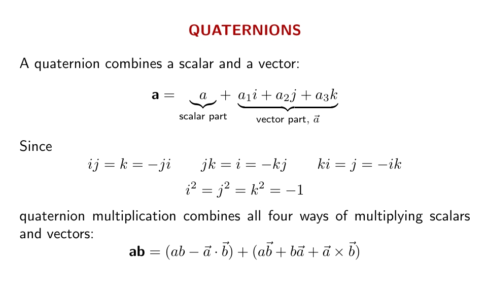
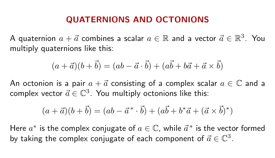
The beauty of quaternion multiplication is that it combines all ways of multiplying scalars and vectors in a single package, with a concept of absolute value that obeys \(|ab| = |a| |b|\).
Last week I realized that octonion multiplication works almost the same way — but with complex scalars and vectors!
An octonion combines a complex number (or 'scalar') and a complex vector in a single package. You multiply them like quaternions, but with some complex conjugation sprinkled in. We need that to get \(|ab| = |a| |b|\) for octonions.
I figured out this formula for octonion multiplication when trying to explain the connection between octonions and the group \(\mathrm{SU}(3)\), which governs the strong nuclear force. You can see details here:
The octonions are to \(\mathrm{SU}(3)\) as the quaternions are to
\(\mathrm{SO}(3)\)! The ordinary dot and cross product are invariant
under rotations, \(\mathrm{SO}(3)\), so the automorphism group of the
quaternions is \(\mathrm{SO}(3)\). For octonions we use complex
vectors, and dot and cross products adjusted to be invariant under
\(\mathrm{SU}(3)\), so the group of octonion automorphisms fixing \(i\)
is \(\mathrm{SU}(3)\).
July 22, 2020
In geometry and topology dimensions 0-4 tend to hog the limelight
because each one is so radically different than the ones before, and
so much amazing stuff happens in these 'low dimensions'.
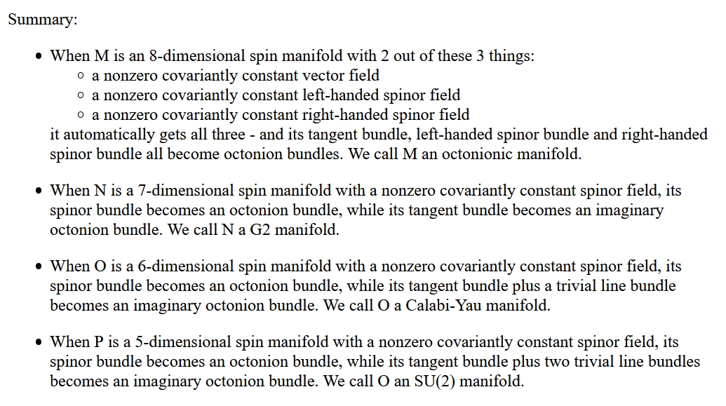
I don't know enough about dimensions 5-7, but... the even part
\(\mathrm{Cliff}_0(n)\) of the Clifford algebra generated by \(n\)
anticommuting square roots of \(-1\) follows a cute pattern for \(n\) =5,6,7:
Real spinors in dimensions 5,6,7 form an 8-dimensional real vector space with extra structure — and more structure as the dimension goes down:
I explain this in a lot more detail in week195 of This Week's Finds:
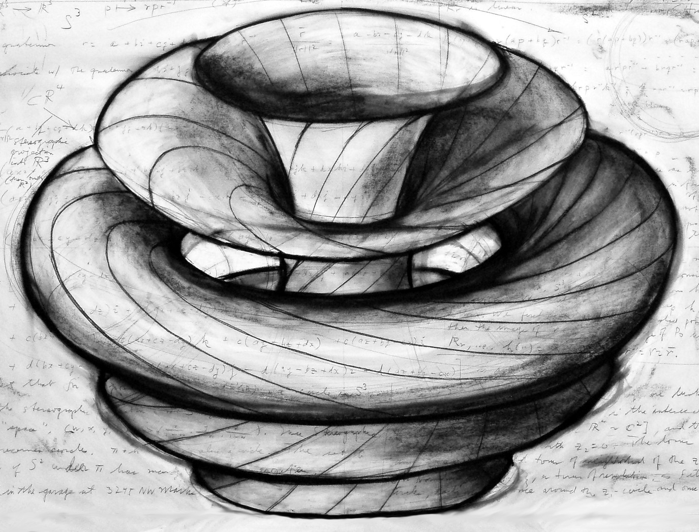
The 3-sphere \(S^3\) can be seen as \(\mathbb{R}^3\) plus a point at infinity. But here London Tsai shows the 'Hopf fibration': \(S^3\) as a bundle of circles over the 2-sphere. Each point in \(S^3\) lies on one circle. The set of all these circles forms a 2-sphere.
\(S^3\) is an \(S^1\) bundle over \(S^2\).
But the 3-sphere \(S^3\) is also a group! It's called \(\mathrm{SU}(2)\): the group of \(2 \times 2\) unitary matrices with determinant \(1\).
So we can see the group \(\mathrm{SU}(2)\) as an \(S^1\) bundle over \(S^2\). But in fact we can build many groups from spheres.
Let's try \(\mathrm{SU}(3)\). This acts on the unit sphere in \(\mathbb{C}^3\). \(\mathbb{C}^3\) is 6-dimensional as a real space, so this sphere has dimension one less: it's \(S^5\). Take your favorite point in here; each element of \(\mathrm{SU}(3)\) maps it to some other point. Using this we can see \(\mathrm{SU}(3)\) is a bundle over \(S^5\).
Many elements of \(\mathrm{SU}(3)\) map your favorite point in \(S^5\) to the same other point. What are they like? They form a copy of \(\mathrm{SU}(2)\), the subgroup of \(\mathrm{SU}(3)\) that leaves some unit vector in \(\mathbb{C}^3\) fixed.
So \(\mathrm{SU}(3)\) is an \(\mathrm{SU}(2)\) bundle over \(S^5\).
But \(\mathrm{SU}(2)\) is itself a sphere, \(S^3\). So \(\mathrm{SU}(3)\) is an \(S^3\) bundle over \(S^5\).
In other words, you can slice \(\mathrm{SU}(3)\) into a bunch of 3-spheres, one for each point on the 5-sphere. It's kind of like a higher-dimensional version of the Hopf fibration shown above.
How about \(\mathrm{SU}(4)\), the \(4 \times 4\) unitary matrices with determinant \(1\)? We can copy everything we just did: this group acts on \(\mathbb{C}^4\) so it acts on the unit sphere in there, which is \(S^7\). The elements mapping your favorite point to some other form a copy of \(\mathrm{SU}(3)\).
So, \(\mathrm{SU}(4)\) is an \(\mathrm{SU}(3)\) bundle over \(S^7\).
Note: we've seen that \(\mathrm{SU}(4)\) is an \(\mathrm{SU}(3)\) bundle over \(S^7\), while \(\mathrm{SU}(3)\) is an \(S^3\) bundle over \(S^5\).
So \(\mathrm{SU}(4)\) is a \(S^3\) bundle over an \(S^5\) bundle over \(S^7\).
Maybe you see the pattern now. We can build the groups \(\mathrm{SU}(n)\) as 'iterated sphere bundles'.
For example, \(\mathrm{SU}(5)\) is an \(S^3\) bundle over an \(S^5\) bundle over an \(S^7\) bundle over \(S^9\).
As a check, you can compute the dimension of \(\mathrm{SU}(5)\) in some other way and show that yes, indeed $$ \dim(\mathrm{SU}(5)) = 3 + 5 + 7 + 9 $$ Even better, the group \(\mathrm{U}(5)\) of all unitary \(5\times 5\) matrices is an \(S^1\) bundle over an \(S^3\) bundle over an \(S^5\) bundle over an \(S^7\) bundle over \(S^9\). The \(S^1\) here comes from the choice of determinant.
So: $$ \dim(U(5)) = 1 + 3 + 5 + 7 + 9 = 5^2 $$ and this pattern works in general.
It's easy to see that the sum of the first \(n\) odd numbers is \(n^2\). But we've found a subtler incarnation of the same fact! We've built \(\mathrm{U}(n)\) out of the first \(n\) odd-dimensional spheres, as an iterated bundle.
image by Vincent Pantaloni
Puzzle. Can you describe \(\mathrm{O}(n)\), the group of
orthogonal \(n \times n\) matrices, as an iterated sphere bundle
in a similar way?
July 26, 2020
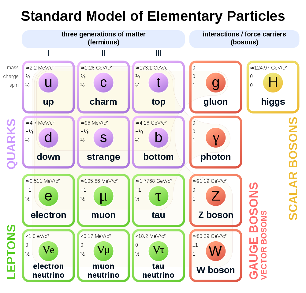
The matter you see is made of up and down quarks, electrons... and then there are electron neutrinos, hard to see. These are the 'first generation' of quarks and leptons.
There are three generations, each with 2 quarks and 2 leptons. Why this pattern?
Short answer: nobody knows.
But we know some stuff.
To get a consistent theory of physics, we need 'anomaly cancellation'. If one generation had just one quark, or a lepton with the wrong charge — and everything else the same — the laws of physics wouldn't work!
Some 'grand unified theories' fit the observed pattern of quarks and leptons quite beautifully. For example, in the \(\mathrm{Spin}(10)\) theory all the quarks and leptons in each generation, and their antiparticles, fit into a neat package: an 'irreducible representation' of this group. This theory forces there to be a quark of electric charge \(+2/3\), a quark of charge \(-1/3\), a lepton of charge \(0\) and a lepton of charge \(-1\) in each generation — which is exactly what we see!
But this theory predicts that protons decay, which we haven't seen (yet?).
A more quirky line of attack, much less well developed, uses octonions. The octonions contain lots of square roots of \(-1\). If you pick one and call it \(i\), the octonions start looking like a quark and a lepton! But only as far as the strong force is concerned.
The strong force has symmetry group \(\mathrm{SU}(3)\). Each quark comes in three 'colors': red, green and blue. This is just a colorful way of saying the quark's quantum states, as far as the strong force is concerned, transform according to the usual representation of \(\mathrm{SU}(3)\) on \(\mathbb{C}^3\).
Each lepton, on the other hand, is 'white'. It doesn't feel the strong force at all. As far as the strong force is concerned, its quantum states transform according to the trivial representation of \(\mathrm{SU}(3)\) on \(\mathbb{C}\).
What does all this have to do with octonions?
Choosing a square root of \(-1\) in the octonions and calling it \(i\) makes them into a complex vector space. The group of symmetries of the octonions that preserve \(i\) is \(\mathrm{SU}(3)\). As a representation of \(SU(3)\), the octonions are \(\mathbb{C} \oplus \mathbb{C}^3\). Just right for a quark and a lepton!
This is not a theory of physics; this is just a small mathematical observation. It could be a clue. It could also be a coincidence. But it's kind of cute.
To give a clear proof of this fact, I came up with a new construction of the octonions using complex numbers:
Then I used that here to get the job done:
So, read those if you're curious about this stuff!
July 28, 2020
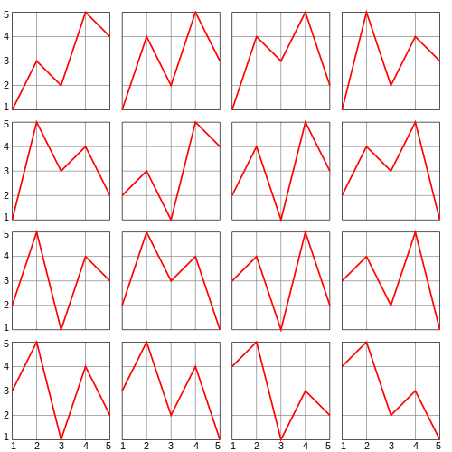
A permutation \(\sigma \colon \{1,\dots,n\} \to \{1,...,n\}\) is alternating if $$ \sigma(1) < \sigma(2) > \sigma(3) < \sigma(4) > \cdots $$ The number of alternating permutations of \(\{1,\dots,n\}\) is called the \(n\)th zigzag number, \(A_n\). For example, the picture above shows \(A_5 = 16\).
The \(n\)th zigzag number equals the \(n\)th coefficient of the Taylor series of \(\sec x\) or \(\tan x\), depending on whether \(n\) is even or odd. This remarkable fact is called André's theorem. You can see one proof here.
Since \(\sec x\) is an even function while \(\tan x\) is odd, we can summarize André's theorem by saying $$ \sum_{n = 0}^\infty \frac{A_n}{n!} x^n = \sec x + \tan x $$
Nice! Trig meets zig.
But here's the weird thing. Take an alternating permutation of \(\{1,\dots,n\}\) and count the triples \(i < j < k\) with \(\sigma(i) < \sigma(j) < \sigma(k)\). The maximum possible value of this count is 0 when \(n<4\), but then it goes like this: $$ 2, 4, 12, 20, 38, 56, 88, \dots $$ Can you spot these numbers in the periodic table?
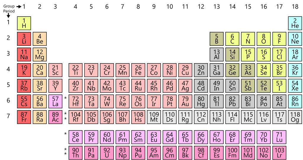
Yes! These numbers, starting with 4, equal the number of electrons in the alkali earth elements: beryllium, magnesium, calcium, strontium, barium, radium,....
Coincidence? No! I don't understand it yet, but it's explained in the new issue of the Notices of the American Mathematical Society — which like any good professional notices, are free to all:
One of the great things about category theory is how it "eats its own tail". Concepts become so general they subsume themselves!
Let me explain with an example: every Grothendieck topos is equivalent to a category of sheaves on itself.
What do all these words mean?
The story starts with complex analysis. Liouville's theorem says every bounded analytic function on the whole complex plane is constant. It follows that every analytic function defined on the whole Riemann sphere is constant.
The interesting analytic functions on the Riemann sphere are just partially defined: for example, they may have poles at certain points. So we need a rigorous formalism to work with partially defined functions.
That's one reason we need sheaves.
There's a 'sheaf' of analytic functions on the Riemann sphere. Call it \(\mathcal{O}\). For any open subset \(U\) of the sphere, \(\mathcal{O}(U)\) is the set of all analytic functions defined on \(U\).
Note if \(V \subseteq U\) we can restrict analytic functions from \(U\) to \(V\), so we get a map \(\mathcal{O}(U) \to \mathcal{O}(V)\).
Even better, we can tell if a function is analytic on an open set \(U\) by looking to see if it's analytic on a bunch of open subsets \(U_i\) that cover \(U\). This says that being analytic is a 'local' property.
Technically: if we have a open set \(U\) covered by open subsets \(U_i\) and analytic functions \(f_i\) on the sets \(U_i\) that agree when restricted to their intersections \(U_i \cap U_j\), there's a unique analytic function on all of \(U\) that restricts to each of these \(f_i\). This is a mouthful, but this is the sheaf condition: the key idea in the definition of a sheaf.
If you understand this example — the sheaf of analytic functions on the Riemann sphere — you can understand the definition of a sheaf on a topological space.
Roughly: for a topological space \(X\), a 'sheaf' \(S\) gives you a set \(S(U)\) for any open \(U \subseteq X\). There's a 'restriction' map $$ S(U) \to S(V) $$ whenever \(V \subseteq U\) is a smaller open set. And a couple of conditions hold — most notably the sheaf condition!
So, sheaves give a rigorous way to study partially defined functions — and more interesting partially defined things — on a topological space. They let us work 'locally' with these entities.
All this was known by the late 1950s. Then Grothendieck came along....
He noticed the open sets of a topological space are the objects of a category. And he showed you could define sheaves on other categories, too!
But to do this you need to choose a 'coverage' (or 'Grothendieck topology') for your category, which says what it means for a bunch of objects to cover another object.
A category with a coverage is called a 'site'. He figured out how to define sheaves on any site. This lets you do math locally... but where the concept of 'location' is no longer an open set, but an object in a category!
The category of all sheaves on a site is called a 'Grothendieck topos'. An example would be the category of all sheaves on the Riemann sphere. Or even simpler: the category of all sheaves on a point! This is just the category of sets.
Grothendieck invented this stuff to help prove some conjectures in algebraic geometry. But Grothendieck topoi took on a life of their own — and in fact, they 'eat their own tail', like the mythical ouroboros.
Notice that categories are showing up in two ways so far:
And the answer is yes! Any Grothendieck topos \(T\) has a god-given coverage making it into a site... and the category of sheaves on this site is equivalent to \(T\) itself.
So it's equivalent to the category of sheaves on itself!
For details go here: