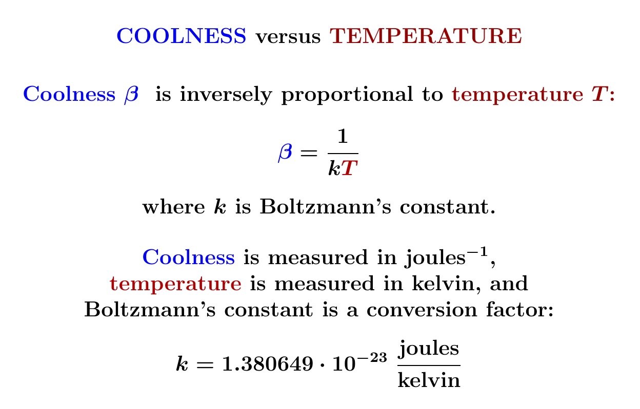
In statistical mechanics, coolness is inversely proportional to temperature. But coolness has units of energy\({}^{-1}\), not temperature\({}^{-1}\). So we need a constant to convert between coolness and inverse temperature! And this constant is very interesting.
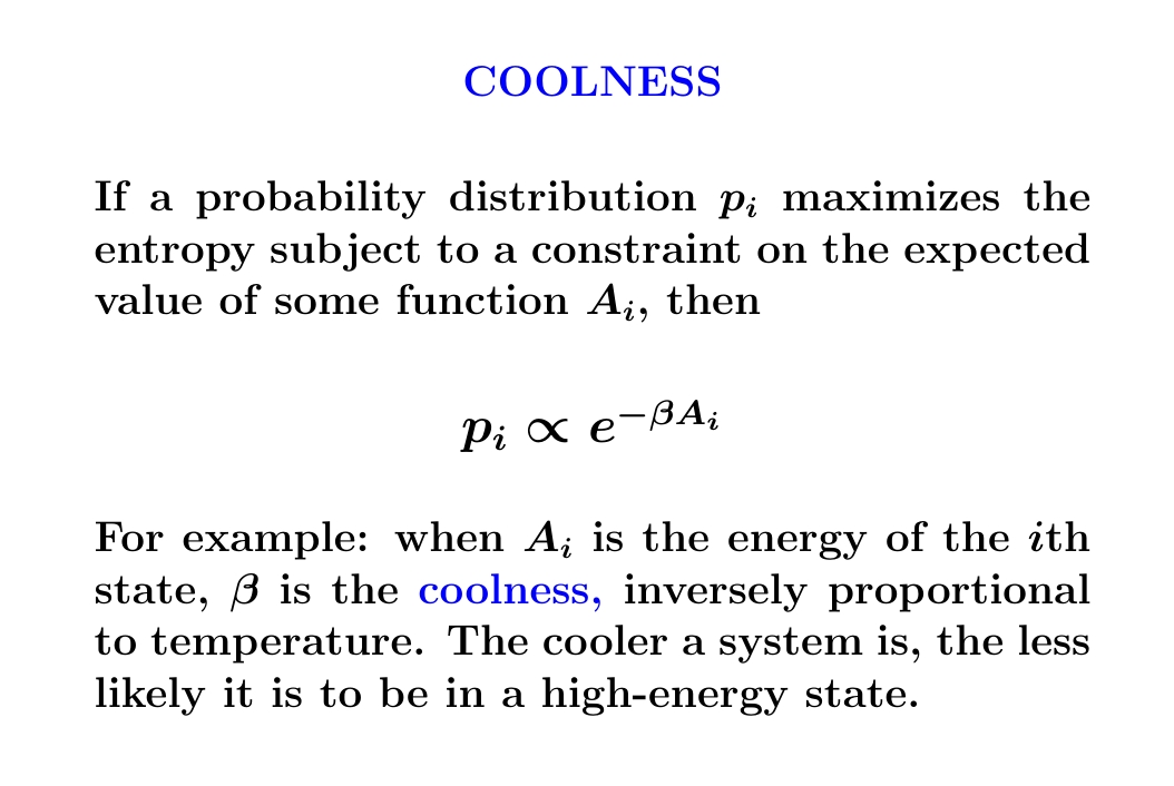
Remember: when a system maximizes entropy with a constraint on its expected energy, the probability of it having energy \(E\) is proportional to \(\exp(-\beta E)\) where \(\beta\) is its coolness. But we can only exponentiate dimensionless quantities! (Why?) So \(\beta\) has dimensions of 1/energy.
Since coolness is inversely proportional to temperature, we must have \(\beta = 1/kT\) where \(k\) is some constant with dimensions of energy/temperature.
It's clear that temperature has something to do with energy... this is the connection!
\(k\) is called 'Boltzmann's constant'. This constant is tiny, about \(10^{-23}\) joules/kelvin. This is mainly because we use units of energy, joules, suited to macroscopic objects like a cup of hot water. Boltzmann's constant being tiny reveals that such things have enormously many microscopic states!
Later we'll see that a single classical point particle, in empty space, has energy \(3kT/2\) when it's maximizing entropy at temperature \(T\). The 3 here is because the atom can move in 3 directions, the \(1/2\) because we integrate \(x^2\) to get this result. The important part is \(kT\). The \(kT\) says: if an ideal gas is made of atoms, each atom contributes just a tiny bit of energy per degree Celsius, roughly \(10^{-23}\) joules. So a little bit of gas, like a gram of hydrogen, must have roughly \(10^{23}\) atoms in it! This is a very rough estimate, but it's a big deal.
Indeed, the number of atoms in a gram of hydrogen is about \(6 \cdot 10^{23}\). You may have heard of Avogadro's number — this is roughly that.
So Boltzmann's constant gives a hint that matter is made of atoms
— and even better, a nice rough estimate of how many per gram!
August 2, 2022
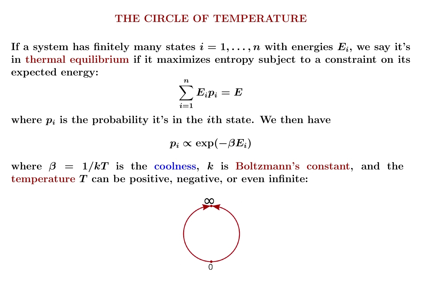
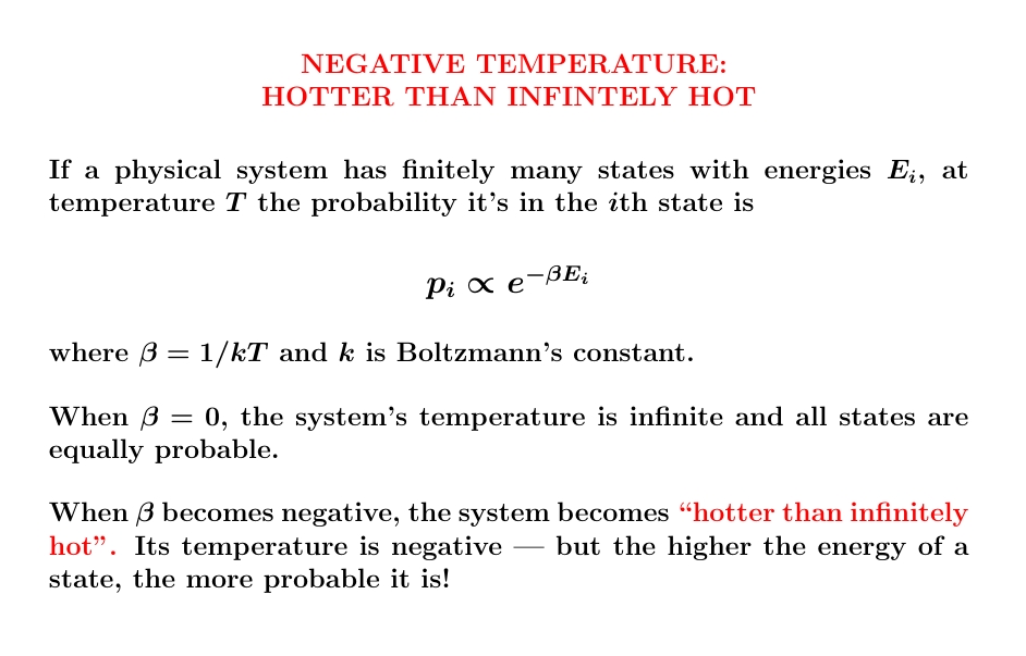
A system with finitely many states can have negative temperature! Even weirder: as you heat it up, its temperature can become large and positive, then reach infinity, and then 'wrap around' and become large and negative!
The reason: the coolness \(\beta = 1/kT\) is more important than the temperature \(T\).
Systems with finitely many states act this way because the sum in the Boltzmann distribution converges no matter what the coolness \(\beta\) equals.
When \(\beta \gt 0\), states with less energy are more probable. When \(\beta \lt 0\), states with more energy are more probable!
For systems with finitely many states, the Boltzmann distribution changes continuously as \(\beta\) passes through zero. But since \(\beta = 1/kT\), this means a large positive temperature is almost like a large negative temperature!
Temperatures 'wrap around' infinity.

However, I must admit the picture of a circle is misleading. Temperatures wrap around infinity but not zero. A system with a small positive temperature is very different from one with a small negative temperature! That's because \(\beta \gg 0\) is very different from \(\beta \ll 0\).
For a system with finitely many states we can take the limit where \(\beta \to +\infty\); then the system will only occupy its lowest-energy state or states. We can also take the limit \(β \to -\infty\); then the system will only occupy its highest-energy state or states.
So, for a system with finitely many states, the true picture of possible thermal equilibria is not a circle but closed interval: the coolness \(\beta\) can be anything in \([-\infty, +\infty]\), which topologically is a closed interval.
In terms of temperature, \(0^+\) is different from \(0^-\).
Now, if all this seems very weird, here's why: we often describe physical systems using infinitely many states, with a lowest possible energy but no highest possible energy. In this case the sum in the Boltzmann distribution can't converge for \(\beta \lt 0\), so negative temperatures are ruled out.
However, some physical systems are nicely described using a finite set of states — or in quantum mechanics, a finite-dimensional Hilbert space of states. Then the story I'm telling today holds true! People study these systems in the lab, and they're lots of fun.
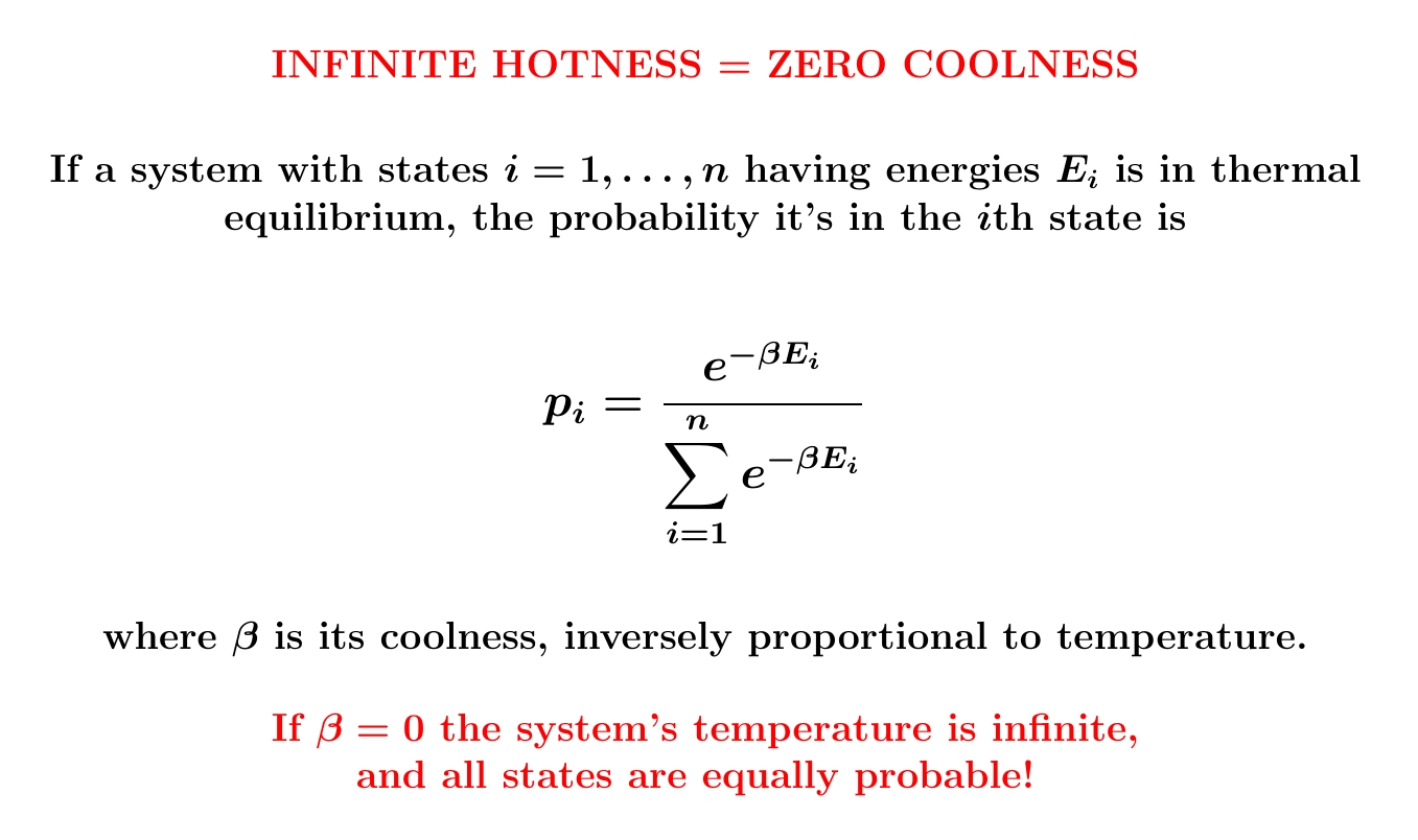
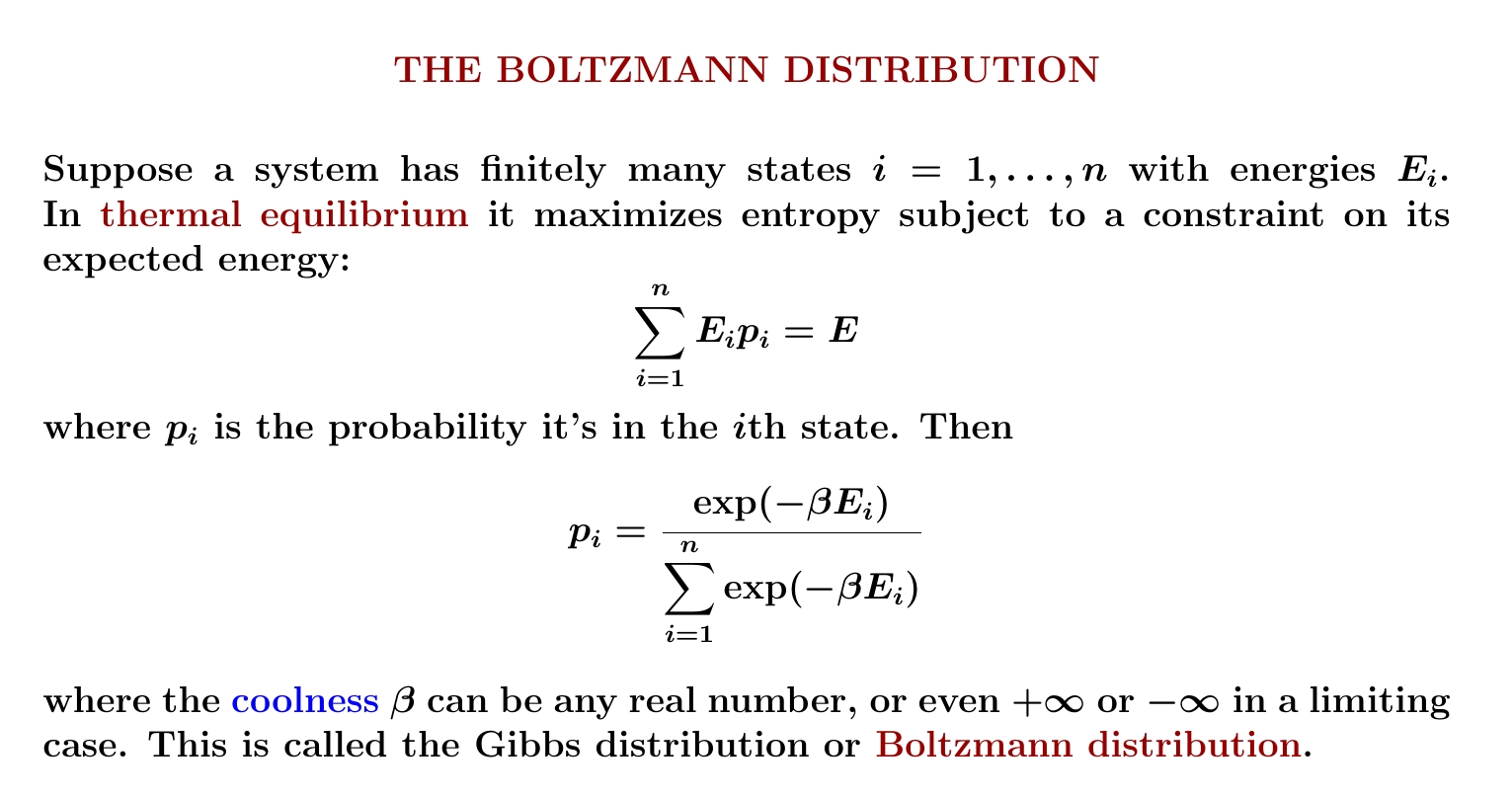
The probability of finding a system in a particular state decays exponentially with energy when the coolness \(\beta\) is positive. But for a system with finitely many states, \(\beta\) can be zero. Then it becomes equally probable for the system to be in any state!
Zero coolness means 'utter randomness': that is, maximum entropy.
Here's why. The probability distribution with the largest entropy is the one where all probabilities \(p_i\) are all equal. This happens at zero coolness! When \(\beta = 0\) we get \(\exp(-\beta E_i) = 1\) for all \(i\). The probabilities \(p_i\) are proportional to these numbers \(\exp(-\beta E_i) = 1\), so they're all equal.
It seems zero coolness is impossible for a system with infinitely many states. With infinitely many states, all equally probable, the probability of being in any state would be zero. In other words, there's no uniform probability distribution on an infinite set.
One way out: replace sums with integrals. For the usual measure \(dx\) on \([0,1]\), each point has the same measure, namely zero, while \(\int_0^1 dx = 1\). So this is a fine 'probability measure' that we could use to describe a system at zero coolness, whose space of states is \([0,1]\).
But replacing sums by integrals raises all sorts of interesting issues. For example, a sum over states doesn't change when you permute the states, but an integral usually does! So a choice of measure is a significant extra structure we're slapping on our set of states.
We'll get into these issues later, since to compute the entropy of an ideal gas using classical mechanics, we'll need integrals! But we'll encounter difficulties, which are ultimately resolved using quantum mechanics.
Anyway: infinite temperature is really zero coolness.
August 4, 2022
A physical system with finitely many states can reach infinite
temperature. It can get even hotter, but then its temperature 'wraps
around' and become negative!
Jacopo Bertolotti has illustrated infinite and negative temperatures in the gif below. It shows a system with finitely many states — the blue lines — with energies ranging from \(0\) to \(E_{\text{max}}\). The number of black dots on a blue line indicates the probability that this system has a specific energy. He shows how this changes as the temperature goes from small positive values up to \(\infty\) and then wraps around to negative values:
His \(k_B\) is Boltzmann's constant, which I'm calling \(k\). What he
calls temperature \(0\), I might call \(0^{+}\), meaning the limit as
\(T\) approaches zero from above. He doesn't take the limit as \(T\)
approaches zero from below: he stops at \(T = -0.1 E_{\text{max}}/k\).
August 11, 2022
I'm learning some crazy things at this conference on logic.
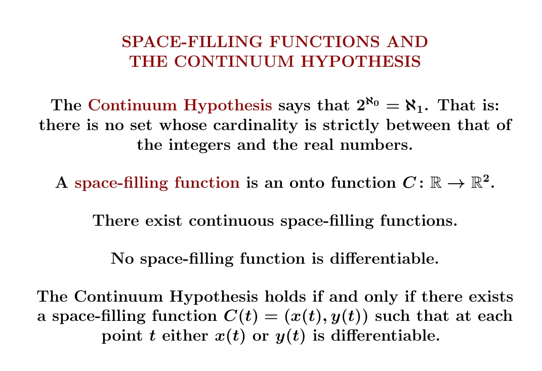
Peano was the first to find a continuous function that maps the closed interval \([0,1]\) onto the square \([0,1]^2\). Later Hilbert found another one. Both these are easiest to describe as a limit of a sequence of continuous functions. Hilbert's example works like this:
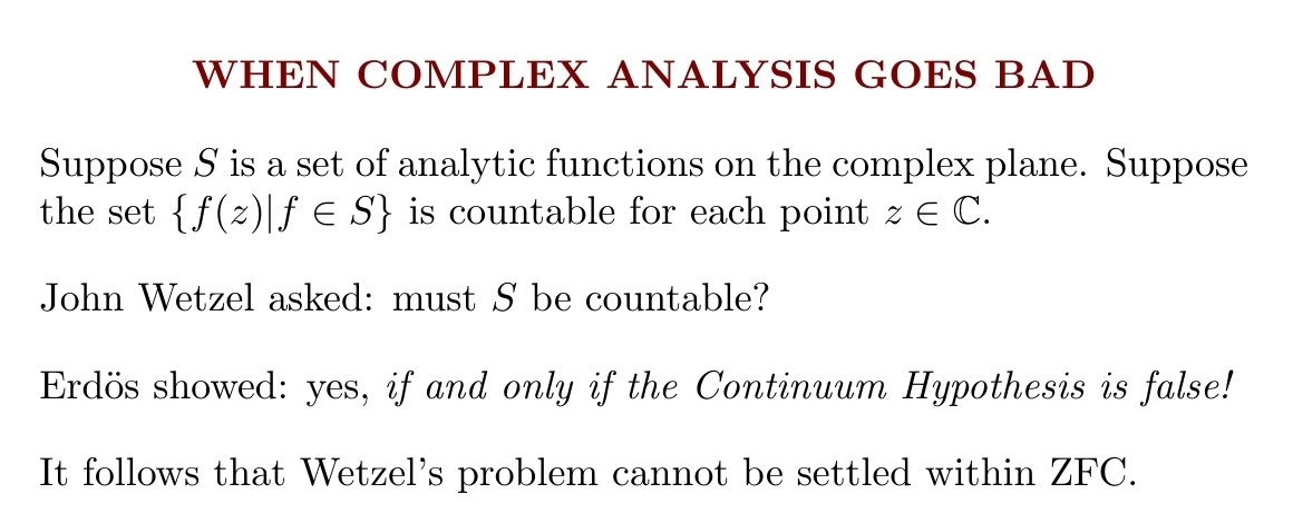
In 1987, Michal Morayne showed the Continuum Hypothesis holds if and only if there's an onto function \(f \colon \mathbb{R} \to \mathbb{R}^2\) such that at each point of \(\mathbb{R}\) at least one component of \(f\) is differentiable. Here's his paper:
If a probability distribution \(p\) maximizes its entropy \(S\) subject only to a constraint on \(\langle E \rangle \), the expected value of its energy, the maximum occurs at a probability distribution \(p\) where $$ d \langle E \rangle = T d S $$ and \(T\) is the temperature. Here's the proof in a picture:

But in fact this formula works for any quantity \(A\), not just energy. And it's clearest if we ignore \(T\) and focus on the Lagrange multiplier \(\beta\).
\(\beta\) also determines the probability distribution where the maximum occurs! The combination of these two formulas is powerful.

The equations here are general mathematical facts, not 'laws of physics' that could be disproved using experiments. They're useful in many contexts, depending on what quantity \(A\) we're studying.
They also generalize to situations where we have more than one constraint.
Here are some more details. The picture here lives in the space of all probability distributions \(p\). I'm drawing \(dS\) as a vector at right angles to a level surface of \(\langle A \rangle\). Really I should draw it as a stack of lines tangent to this level surface! The differential \(dS\) is a 1-form, the vector is the gradient \(\nabla S\).

The idea, which should be familiar if you've studied Lagrange multipliers, is that when when we maximize a function \(f\) subject to a constraint \(g = \mathrm{constant}\), the gradient of \(f\) must point at right angles to the surface \(g = \mathrm{constant}\). Or, in terms of 1-forms, \(df = \beta\, dg\) for some number \(\beta\). Here this idea is giving us \(d S = \beta \, d\langle A \rangle\).
How do we get the formula $$ p_i = \frac{\exp(-\beta A_i)}{\sum_{i=1}^n \exp(-\beta A_i)} ? $$ This is an important calculation, and you can see it done here:
In the current version of this calculation, at one step they say "apply the first law of thermodynamics". That's a wee bit misleading, so I hopes someone fixes it. We can do the whole calculation using just math: the Lagrange multiplier they call \(-\lambda_2\) is what I'm calling \(\beta\) The "first law of thermodynamics" is only used to rename this quantity \(1/kT\), where \(k\) is Boltzmann's constant.I prefer to maximize entropy with a constraint on the expected value of an arbitrary quantity \(A\): this is just math. Then we can argue that when \(A\) is energy, the Lagrange multiplier \(\beta\) deserves to be called 'coolness'. I made that argument back on July 27th.

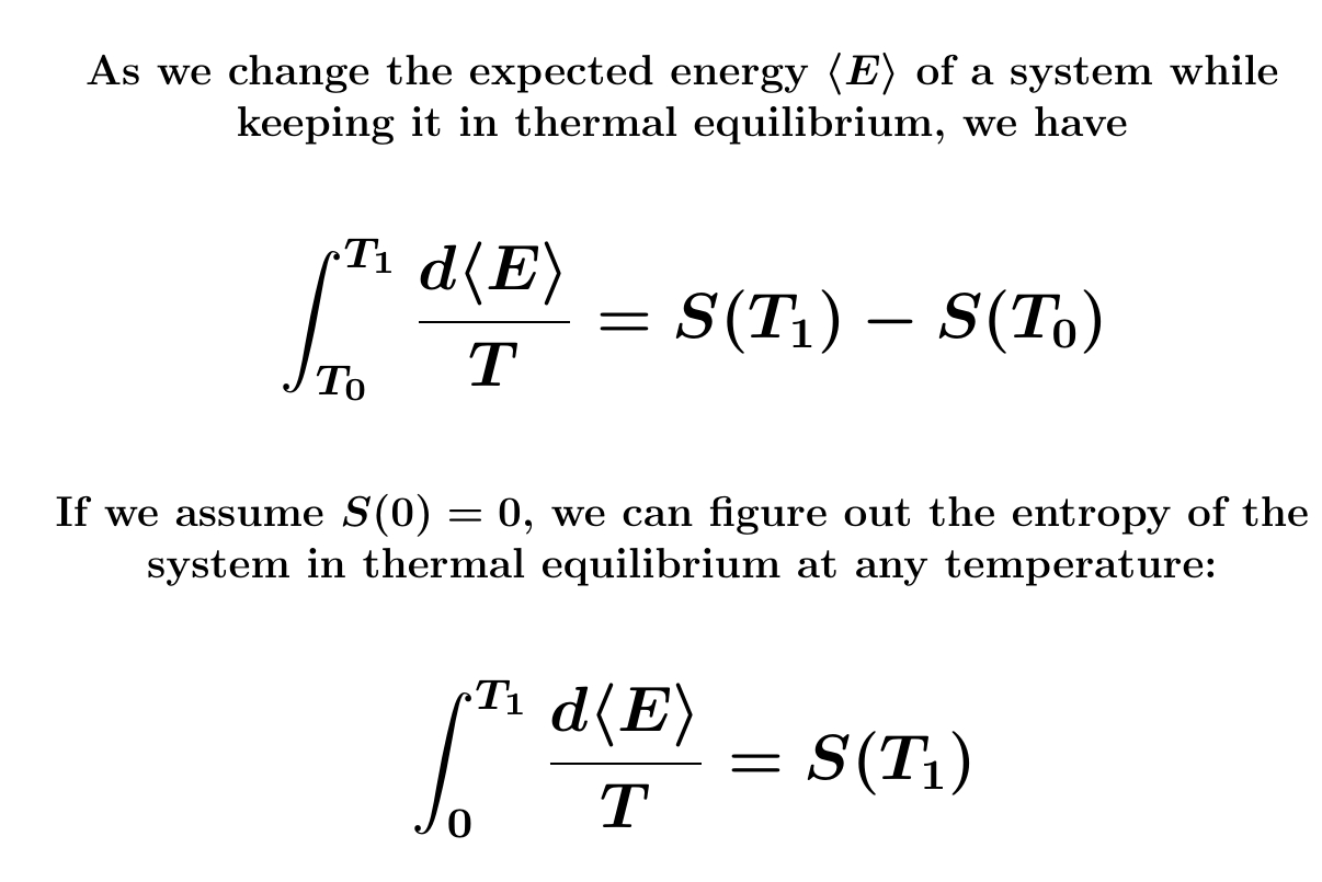
It's hard to measure entropy. But we know how entropy changes as we slowly warm or cool a system while keeping it in thermal equilibrium! This helps a lot.
('Thermal equilibrium' is the probability distribution that maximizes \(S\) for a given expected energy \(\langle E \rangle\).
Suppose a system in thermal equilibrium has no entropy when the temperature is absolute zero. More about that later.) Then we can figure out its entropy at higher temperatures by slowly warming it, keeping it approximately in thermal equilibrium, and totaling up \(d \langle E \rangle / T \).
People actually do this! So they've figured out the entropy of many substances at room temperature — really 298.15 kelvin — and standard atmospheric pressure. They usually report the answers in joules/kelvin per mole, but I enjoy "bits per molecule".

A mole is about \(6.022 \times 10^{23}\) molecules — this is called Avogadro's number. A joule/kelvin is about \(7.2421 \times 10^{22}\) nats — this is the reciprocal of Boltzmann's constant. A bit is \(\ln 2\) nats.
Using all this, we see 1 joule/kelvin per mole is about \(0.1735\) bits/molecule.
Here's a table of entropies:
My goal all along in this course has been to teach you how to compute some of these entropies (approximately) from first principles... and understand how entropy is connected to information.
We're getting close!
August 16, 2022
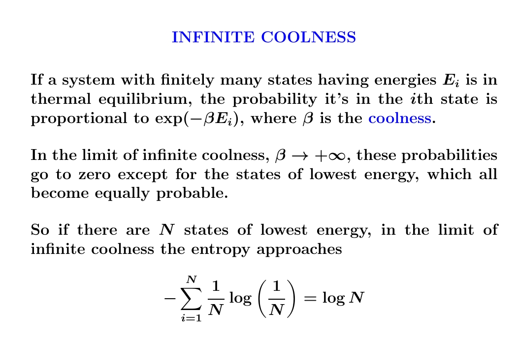
It seems impossible to reach absolute zero. But as you get closer, the entropy of a system in thermal equilibrium approaches \(\log N\), where \(N\) is the number of lowest-energy states. So if it has just one lowest-energy state, its entropy approaches zero.
So, if a system has just one lowest-energy state, we can estimate its entropy in thermal equilibrium at any temperature! We track how much energy it takes to warm it up to that temperature, keeping it close to equilibrium as we do, and use this formula:
But beware: for systems with lots of low energy states, like 'spin glasses', their entropy in thermal equilibrium can be large even near absolute zero! Also, a related problem: systems may take a ridiculously long time to reach equilibrium!
For example, diamond is not the equilibrium form of carbon at room temperature and pressure — it's graphite! But it takes at least billions of years for a diamond to slowly turn to graphite. In fact I've never seen a credible calculation of how long. So, you have to be careful when applying statistical mechanics.
For more subtleties concerning the 'residual entropy' of a material - its entropy near absolute zero — start here:
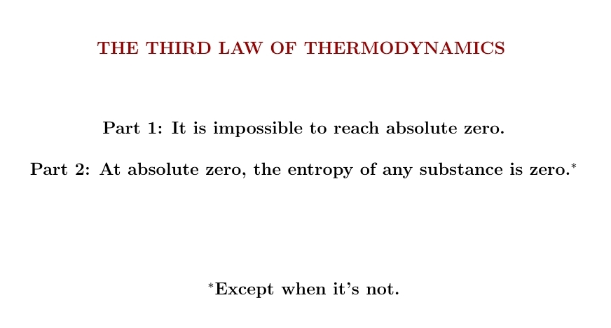
The Third Law of Thermodynamics is a bit odd. People don't agree on what it says; one version seems to undercut the other — and some people add qualifications that weaken it. In 1912 Walther Nerst stated it roughly this way: it is impossible for any procedure to make a system reach zero temperature in a finite number of steps. A more popular version says that the entropy of a system approaches zero as the temperature approaches zero from above. This has the advantage of following from the Boltzmann distribution if the system has one state of lowest energy and the sum in the Boltzmann distribution converges for small positive temperatures — that is, large positive \(\beta\).
To make sure the system has just one state of lowest energy, some people restrict the Third Law to perfect crystals. For example Gilbert N. Lewis and Merle Randall stated it this way in 1923:
If the entropy of each element in some (perfect) crystalline state be taken as zero at the absolute zero of temperature, every substance has a finite positive entropy; but at the absolute zero of temperature the entropy may become zero, and does so become in the case of perfect crystalline substances.
Read Wikipedia for more takes on the Third Law. Currently the first version they state is quite weak: it says entropy approaches some constant value as \(T \to 0\) from above. Then, as a kind of footnote, they say this constant doesn't depend on the pressure, etc. I think that's just false.
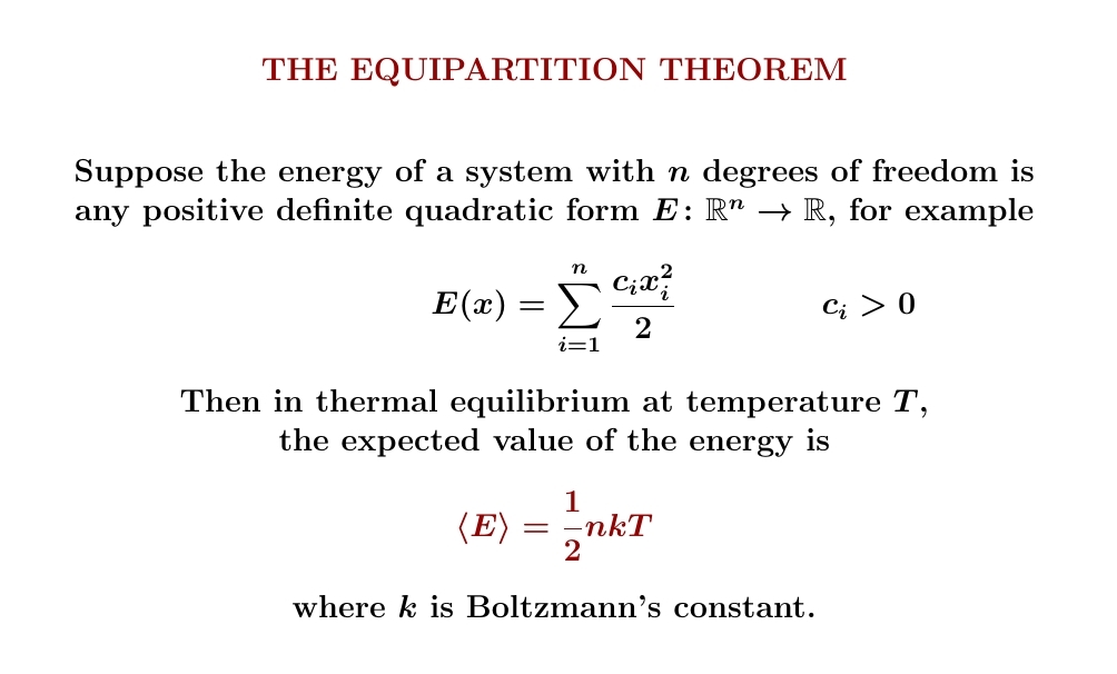
Temperature is very different from energy. But sometimes — just sometimes — the expected energy of a system in thermal equilibrium is proportional to its temperature. The equipartition theorem says happens when the energy depends quadratically on several real variables, defining a positive definite quadratic form on \(\mathbb{R}^n\). For example, it happens for a classical harmonic oscillator.
Let's prove it!
But to prove a theorem, you have to understand the definitions. Here is some background:

We're defining entropy with an integral now, unlike a sum as before, and sticking Boltzmann's constant into the definition of entropy, as physicists do, so that entropy has units of energy over temperature.
Given the formula for the energy \(E\) as a function on \(\mathbb{R}^n\), we'll have to find the Gibbs distribution and then compute \(\langle E \rangle\) as a function of \(T\).
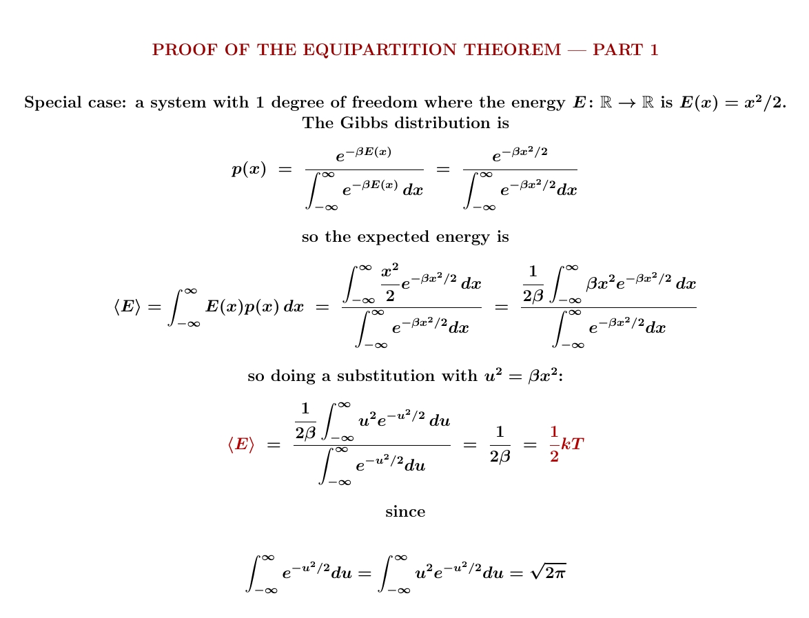
We'll do two special cases before proving the general result. First let's do a system with 1 degree of freedom where the energy is \(E(x) = x^2/2\). In this case, after a change of variables, the Gibbs distribution becomes a Gaussian with mean 0 and variance 1, and that gives the desired result. Or just do the integrals and see what you get! The expected energy \(\langle E \rangle \) is \(\frac{1}{2}kT\).
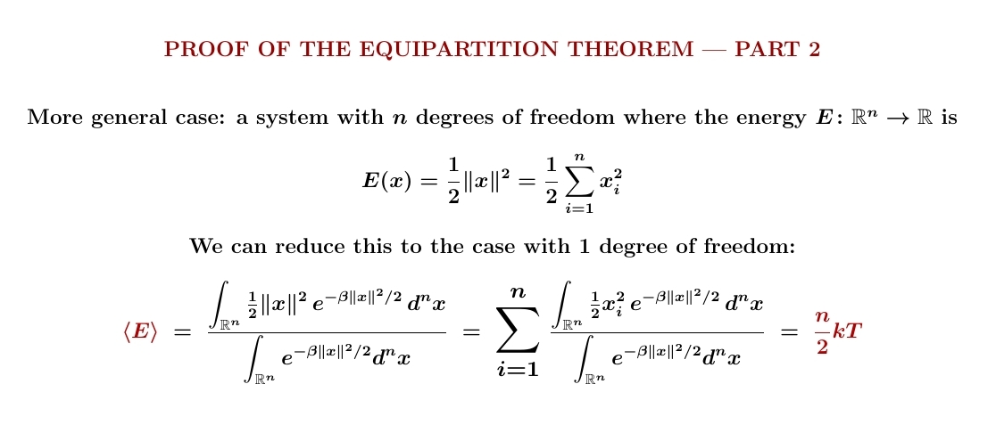
Next let's do a system with \(n\) degrees of freedom where the energy is a sum of \(n\) terms of the form \(x_i^2/2\). It's no surprise that each degree of freedom contributes \(\frac{1}{2}kT\) to the expected energy, giving $$ \langle E \rangle = \frac{1}{2} nkT $$ But make sure you follow my calculation. I skipped a couple of steps!
Finally let's do the general case! We can reduce this to the previous case with a change of variables, so we still get $$ \langle E \rangle = \frac{1}{2} nkT $$ So, each degree of freedom still contributes \(\frac{1}{2}kT\) to the expected energy. That's the equipartition theorem!
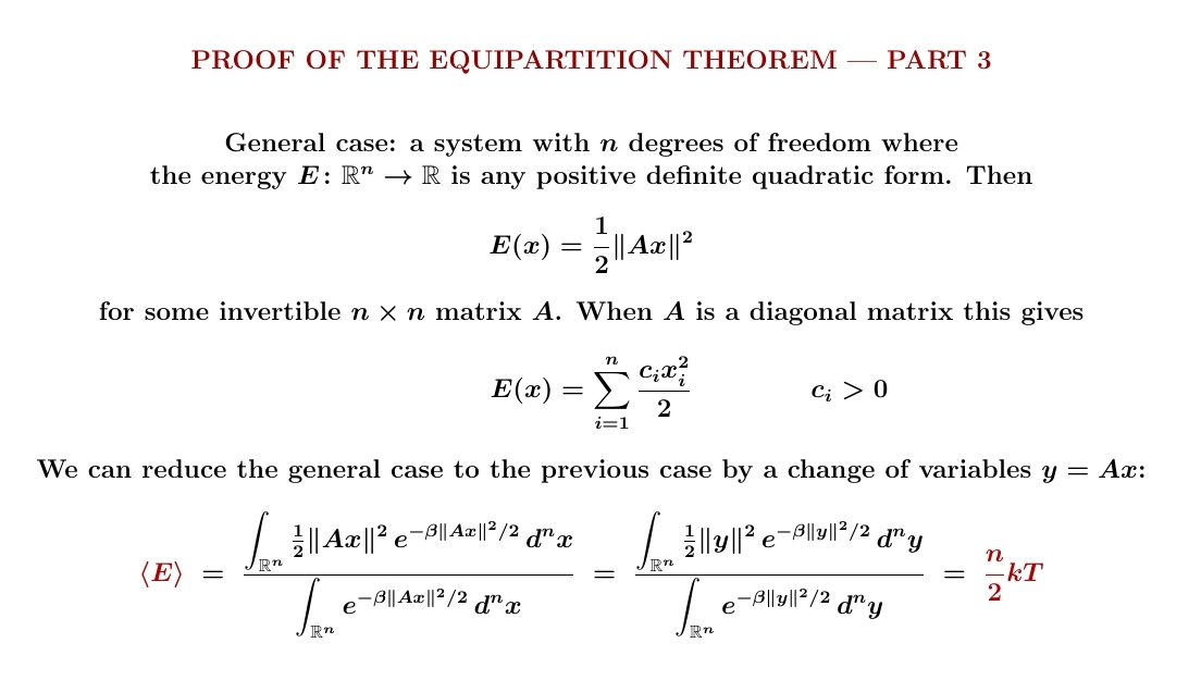
But be careful: some people get carried away. The equipartition theorem stated here doesn't apply when the energy is an arbitrary function of \(n\) variables! It also fails when we switch from classical to quantum statistical mechanics! That's how Planck dodged the ultraviolet catastrophe that occurs classically when \(n \to \infty\).

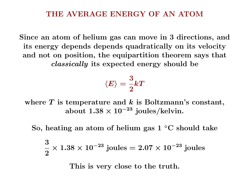
Of course we don't heat up an individual atom: we heat up a bunch. A mole is \(6.02 \times 10^{23}\) atoms, so heating up a mole of helium one degree Celsius (= 1 kelvin) should take about $$ 6.02 \times 10^{23} \times 2.07 \times 10^{-23} \approx 12.46 \textrm{ joules} $$ And this is very close to correct! It seems the experimentally measured answer is \(12.6\) joules.
What are the sources of error? Most importantly, our calculation neglects the interaction between helium atoms. Luckily this is very small at room temperature and pressure. We're also neglecting quantum mechanics. Luckily for helium this too gives only small corrections at room temperature and pressure.
It's important here that helium is a monatomic gas. In
hydrogen, which is a diatomic gas, we
get extra energy because this molecule can tumble around, not just
move along. We'll try that next.
August 20, 2022
A molecule of hydrogen gas is a blurry quantum thing, but let's
pretend it's a classical solid dumbbell that can move and tumble but
not spin around its axis. Then it has 3+2 = 5 degrees of freedom, and
we can use the equipartition theorem to estimate its energy.
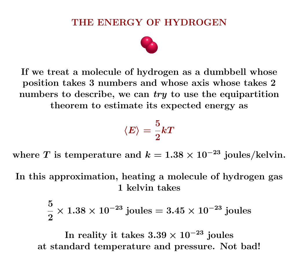
For \(T\) significantly less than 6000 kelvin, hydrogen molecules don't vibrate as shown below. They don't spin around their axis until even higher temperatures. But they tumble like a dumbbell as soon as \(T\) gets exceeds about 90 kelvin.
We need quantum mechanics to compute these things. But at room temperature and pressure, we can pretend a hydrogen gas is made of classical solid dumbbells that can move around and tumble but not spin around their axes! In this approximation the equipartition theorem tells us \(\langle E \rangle = \frac{5}{2} kT\).
I still need to compute the entropy of hydrogen and helium.
For the continuation of this tale, go to my
September 4th diary entry!
August 22, 2022
I'm helping people write software for modeling epidemic disease
— using categories. How does category theory help? It gives
tools for building complex models out of smaller pieces.
Here I explain the history of this work, and the actual math:
Category theory helps us model 'open systems': systems where stuff - matter, energy, information, etc. — flow in and out through a boundary. It gives a very general but practical framework for putting together open systems to form bigger ones.

In epidemiology, people often model disease using 'stock-flow diagrams', showing how people get sick, go to the hospital, acquire resistance, lose it, etc. These diagrams get really big and complicated! So we built software for assembling them from smaller pieces.

It's easy enough to define stock-flow diagrams mathematically — here's the simplest kind, and a little example where the 'stocks' are Susceptible, Infected, Resistant and Dead:

But category theory lets us work with 'open' stock-flow diagrams.
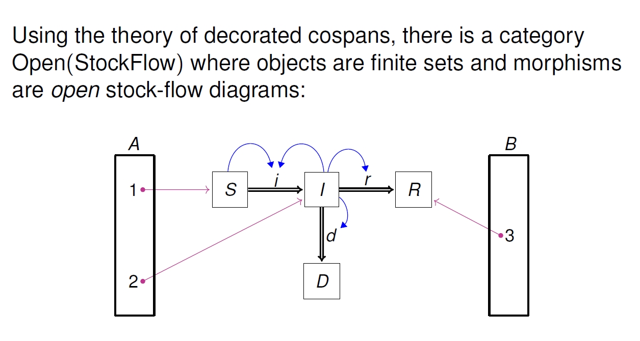
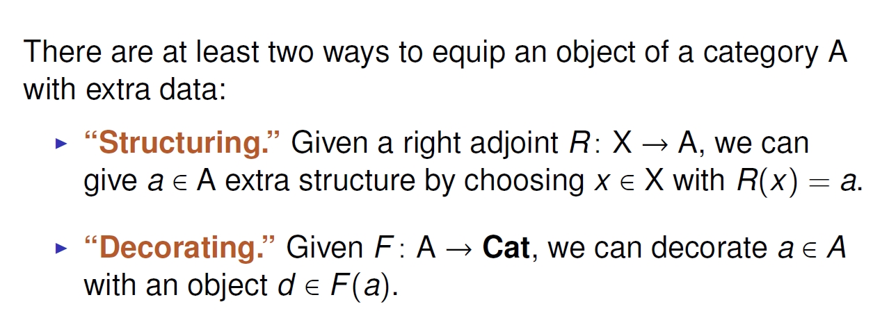
To work with open stock-flow diagrams, it helps to have a general theory of open systems, and how the boundary is related to the system itself. In fact we have two, called 'decorated cospans' and 'structured cospans'. My talk explains these and how they're related.
To see how these abstract ideas get applied to epidemic modeling, try this other talk of mine:
Or read our paper:
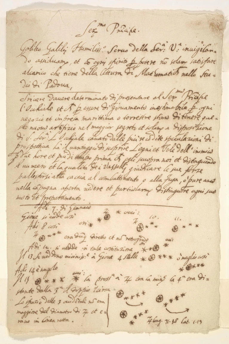
This famous manuscript, supposedly containing Galileo's observations of Jupiter's moons, may be a fake! It was given to the Archbishop of Pisa by a well-known forger who was later convicted of selling a fake Mozart autograph. And now more evidence has turned up: it turns out to have a watermark — "BMO", standing for the Italian city of Bergamo &mdash that has only been seen elsewhere after 1770. That's 150 years after Galileo saw Jupiter's moons! The librarians at the University of Michigan who hold this manuscript now think it's a forgery.
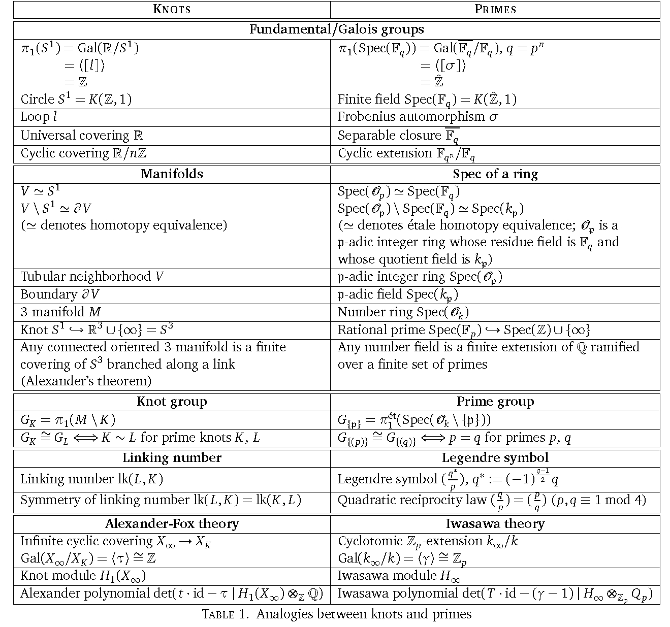
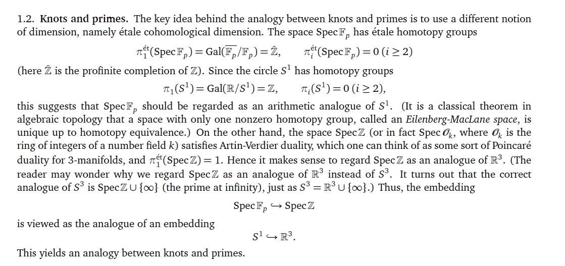
A mystery I keep trying to understand is the analogy between knots and primes. People keep making bigger and bigger charts like this, but you need to know a lot of topology and number theory to understand them. I'm slowly catching up on the number theory side.
I got this chart from Chao Li and Charmaine Sia's excellent course notes:
When you understand this stuff, you'll understand how two primes can be 'linked'. The Legendre symbol of two primes is analogous to the linking number of two knots.
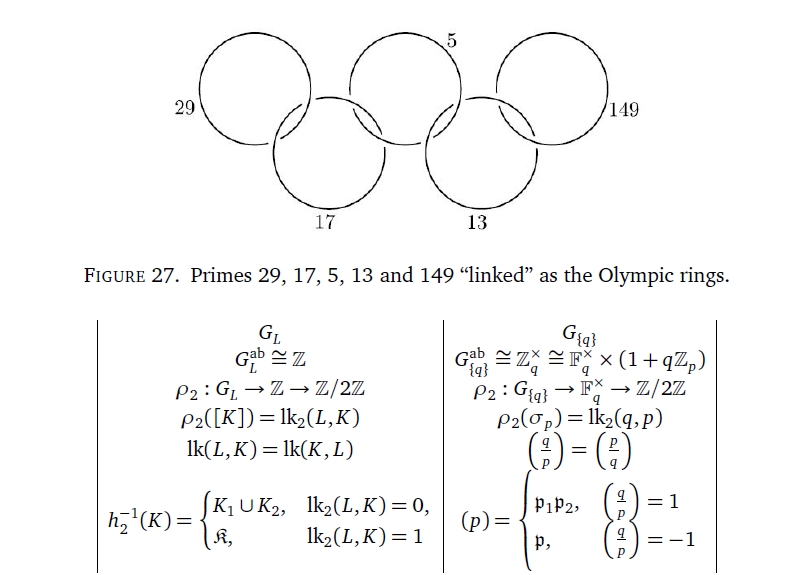
To get deeper into this I'm needing to learn some étale cohomology. This reveals that the ring of integers is 3-dimensional in a certain way, while each prime resembles a circle. The map from \(\mathbb{Z}\) to the field with \(p\) elements for a prime \(p\) is like an embedding of the circle in \(\mathbb{R}^3\).