
This 'paradox' is like a baby version of the ultraviolet catastrophe — not as hard to solve.
We need to look more carefully at the three rules we used to get this 'paradox', and find a way out.
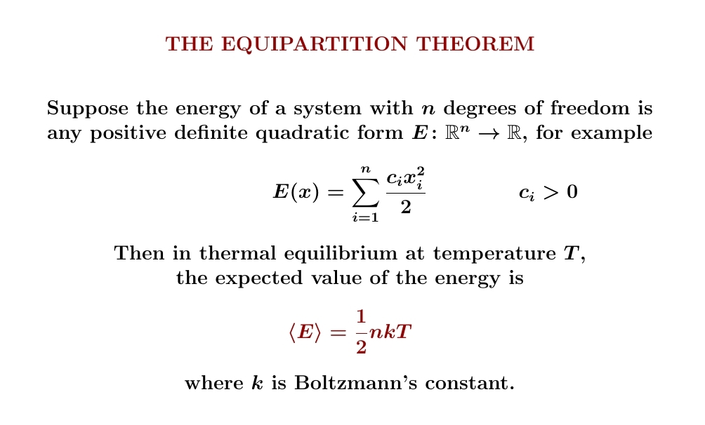
The equipartition theorem applies only under certain special conditions. We studied this on August 18th. For example, it applies to a molecule of a classical ideal gas. But no gas is ideal at very low temperatures. Is that the way out?
On August 15th we derived the relation \(d \langle E \rangle = TdS\) for systems with finitely many states, where entropy is a sum. But we derived the equipartition theorem for certain systems with infinitely many states, where entropy is an integral! Is that the problem?

On August 16th we proved the Third Law — entropy vanishes at zero temperature — for systems with finitely many states and a single state of lowest energy. But the equipartition theorem holds only for certain systems with infinitely many states! Is that the problem?
If we mainly care about actual gases, the best way out is to admit that the equipartition theorem doesn't apply at low temperatures, when the gases become liquid or even solid, and quantum mechanics matters a lot. The Third Law and \(d \langle E \rangle = TdS\) still hold.
But suppose we care about a purely theoretical system described using classical statistical mechanics, obeying all the conditions of the equipartition theorem. Then we should admit that the Third Law doesn't apply to such a system! In fact \(S \to -\infty\) as \(T \to 0\).
Since this is a course on classical statistical mechanics, I want to to compute the entropy of a classical system obeying the conditions of the equipartition theorem, like a single molecule of an ideal gas, or a harmonic oscillator. When we do this, we'll see \(S \to -\infty\) as the temperature approaches zero.
This is just one of the problems with the classical ideal gas,
solved later using quantum mechanics!
September 6, 2022
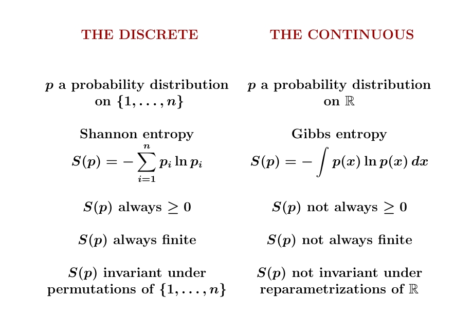
You can switch from finite sums to integrals in the definition of entropy, but be careful: a bunch of things change! When you switch to integrals, the entropy can be negative, it can be infinite — and most importantly, it depends on your choice of coordinates.
I already showed on September 4th that
negative Gibbs entropy arises in any classical system that obeys the
equipartition theorem, like a classical harmonic oscillator or ideal
gas. Its entropy becomes negative at low temperatures!
September 9, 2022

What's the entropy of a classical harmonic oscillator in thermal equilibrium? We can compute it... or we can think a bit, and learn a lot with much less work.
It must grow logarithmically with temperature! But there's an unknown constant \(C\) here. What is it?
We can make progress with a bit of dimensional analysis. The quantity \(\ln T\) is a funny thing: if we change our units of temperature, it changes by adding a constant! So \(k \ln T\) doesn't have dimensions of entropy. But $$ S = k (\ln T + C) $$ must have dimensions of entropy. The constant \(C\) must save the day!

For dimensional reasons, the constant \(C\) must equal \(-\ln T_0\) for some temperature \(T_0\) that we can compute for any harmonic oscillator. What is \(T_0\)? We could just compute it. But it's more fun to use dimensional analysis.
What could it depend on? Obviously the mass \(m\), the spring constant \(\kappa\) and Boltzmann's constant \(k\).
But there's no way to form a quantity with units of temperature from just \(m, \kappa\) and \(k\). So we need an extra ingredient.
And we've seen this already: to define the entropy of a probability distribution on the \(p,q\) plane and get something with the right units, we need a quantity with units of action! The obvious candidate is Planck's constant \(\hbar\), and this is actually right. The entropy we're after is given by an integral with respect to \(dp\, dq / h\) where \(\hbar = h/ 2 \pi\). So the temperature \(T_0\) can depend on \(\hbar\) as well as \(m, \kappa\) and \(k\).
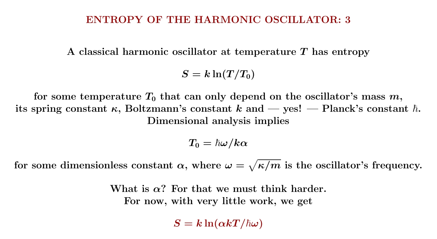
We can compute a quantity with units of temperature from \(m, \kappa, k\) and \(\hbar\). The frequency of our oscillator is \(\omega = \sqrt{k/m} \), and it's a famous fact that \(\hbar \omega\) has units of energy. \(k\) has units of energy/temperature... so \(\hbar\omega/k\) units of temperature!
Using dimensional analysis, we can see the only choice for our temperature \(T_0\) is \(\hbar \omega/k\) times some dimensionless purely mathematical constant, which I'll call \(1/\alpha\). \(\alpha\) must be something like \(\pi\) or \(2\pi\), or if we're really unlucky, \(e^{666}\) — though practice that never seems to happen.
So, the entropy of a classical harmonic oscillator must be $$ S = k \ln(T/T_0) = k \ln(\alpha kT/\hbar \omega). $$
This is far as I can get without breakng down and doing some real work. Later I will compute \(\alpha\).
In summary, here is where we've gotten so far:

But this is already very interesting! \(kT\) is known to be the typical energy scale of thermal fluctuations at temperature \(T\). \(\hbar \omega\) is the spacing between energy levels of a quantum harmonic oscillator with frequency \(\omega\).
What does the ratio \(kT/\hbar\omega\) mean?
\(kT/\omega\hbar\) is roughly the number of energy eigenstates in which we may find a quantum harmonic oscillator with high probability when it's at temperature \(T\). In Boltzmann's old theory of entropy, we just take the logarithm of this number and multiply by \(k\) to get the entropy! This crude calculation gives \(S \approx \ln(kT/\hbar\omega)\). We've seen that classically \(S = \ln(\alpha kT/\hbar\omega)\) for some constant \(\alpha\).

Yesterday we found a formula for the entropy of a classical harmonic oscillator... which includes a mysterious purely mathematical dimensionless constant \(\alpha\). Now let's figure out \(\alpha\).
We'll grit our teeth and actually do the integral needed to calculate the entropy — but only in one easy case! Combining this with our formula, we'll get \(\alpha\).
First, recall the basics. The energy \(E(p,q)\) of our harmonic oscillator at momentum \(p\) and position \(q\) determines its Gibbs distribution at temperature \(T\), which I'll call \(\rho(p,q)\) now since the letter \(p\) is already used. Integrating \(-\rho \ln \rho\) we get the entropy. In physics we multiply this by Boltzmann's constant to get the units right. Entropy has units of energy/temperature, and 1 nat of entropy is about \(1.38 \times 10^{-23}\) joules/kelvin, which is Boltzmann's constant \(k\). So \(k\) equals 1 nat.

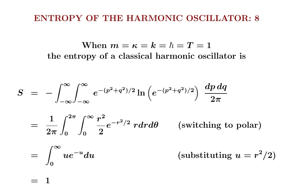
Let's compute the Gibbs distribution \(\rho(p,q)\) and the entropy \(S\). To keep the formulas clean, we'll work in units where \(m = \kappa = k = \hbar = 1\), and compute everything at one special temperature: \(T = 1\).
In this case \(h = 2\pi\), and \(\rho(p,q)\) is a beautiful Gaussian whose integral \(dp dq\) is \(2\pi\). These two factors of \( 2\pi \) cancel, so \(\rho(p,q) = e^{-(p^2 + q^2)/2}\).

Now let's do the integral to compute the entropy! We use a famous trick for computing the integral of a Gaussian: switching to polar coordinates and then a substitution \(u = r^2/2\). But for us \(r^2/2\) is minus the logarithm of the Gaussian!
After all this work, we get \(S = 1\).
Knowing the entropy in this one special case, we can figure out the mysterious constant \(\alpha\) in our general formula for the entropy:
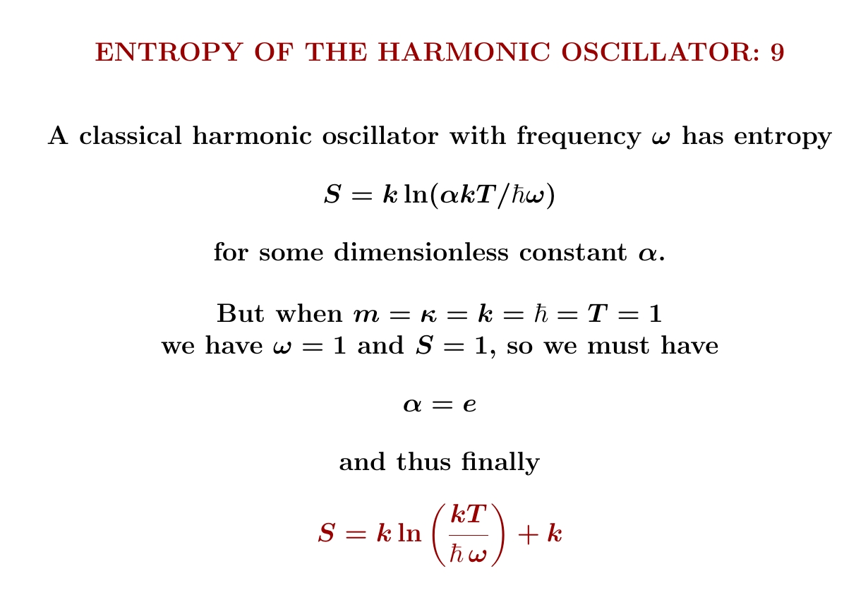
We see \(\alpha\) must equal \(e\). So, the entropy of an oscillator
with frequency \(\omega\) at temperature \(T\) is
$$ S = k \ln(ekT/\hbar\omega) = k \ln(kT/\hbar \omega) + k $$
The extra \(k\) here is fascinating to me. If we had slacked off,
ignored the possibility of a dimensionless constant \(\alpha\), and crudely
used dimensional analysis to guess \(S\) approximately the way people
often do, we might have gotten
$$ S = k \ln(kT/\hbar\omega) $$
This would be off by 1 nat. What does the 1 extra nat mean?
To be frank I don't know yet.
September 18, 2022
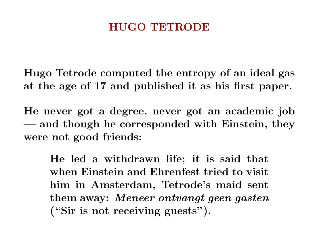
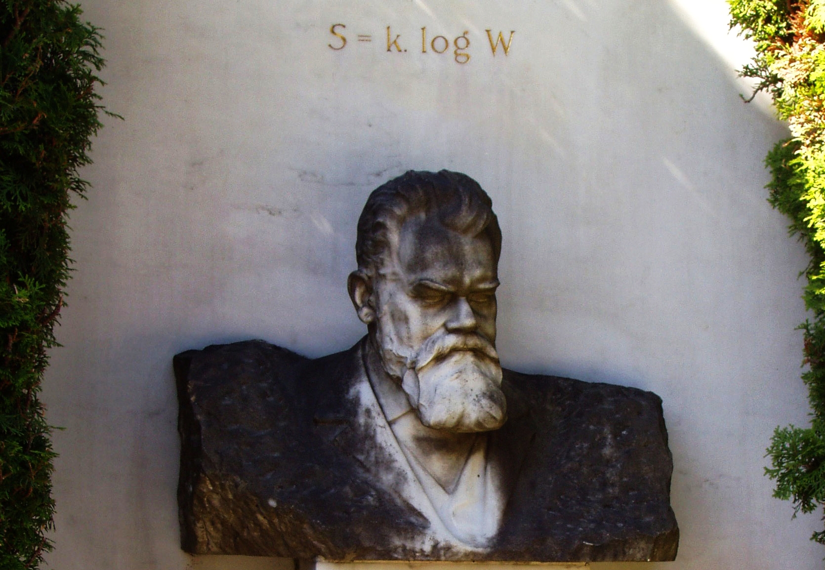
The goal of my 'course' here is for you to understand the entropy of an ideal gas. Sackur and Tetrode computed this in 1912. Sackur wrote two papers with mistakes in them. Tetrode got it right the first time!
He's an interesting guy.
As you might guess from the story, Tetrode came from a rich family: his dad was the director of the Dutch National Bank.
In 1928 he wrote a paper combining the Dirac equation and general relativity, "General-relativistic quantum theory of electrons":
But why did Einstein try to see him before 1928?
The Sackur–Tetrode equation for the entropy of an ideal gas, which I'll explain later, involves statistical mechanics and Planck's constant — right up Einstein's alley. Then in 1922 Einstein read this paper by Tetrode:
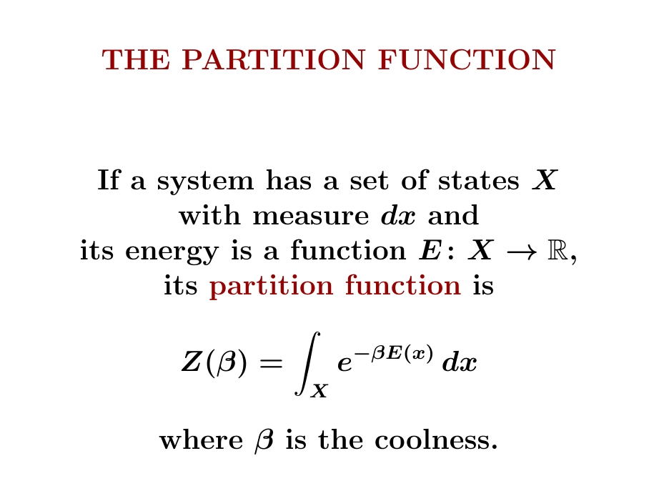
I want to compute the entropy of a particle in a box. I could do it directly, but that's a bit ugly. It's better to use the 'partition function'. This amazing function knows everything about statistical mechanics. From it you can get the entropy — and much more!
The partition function is the thing you have to divide \(e^{-\beta E(x)}\) by to get a function whose integral is 1: the Gibbs distribution, which is the probability distribution of states in thermal equilibrium at coolness \(\beta\).
A humble normalizing factor! And yet it becomes so powerful. Kind of surprising.

Next time I'll show you how to compute the expected energy \(\langle E \rangle\) and the entropy \(S\) of any system starting from its partition function.
Like Lagrangians, it's easy to use partition functions, but it's hard to say what they 'really mean'.
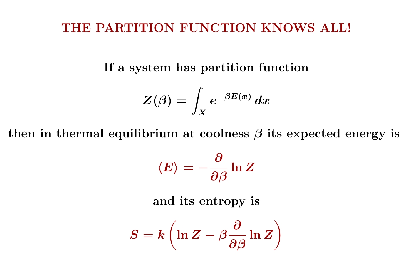
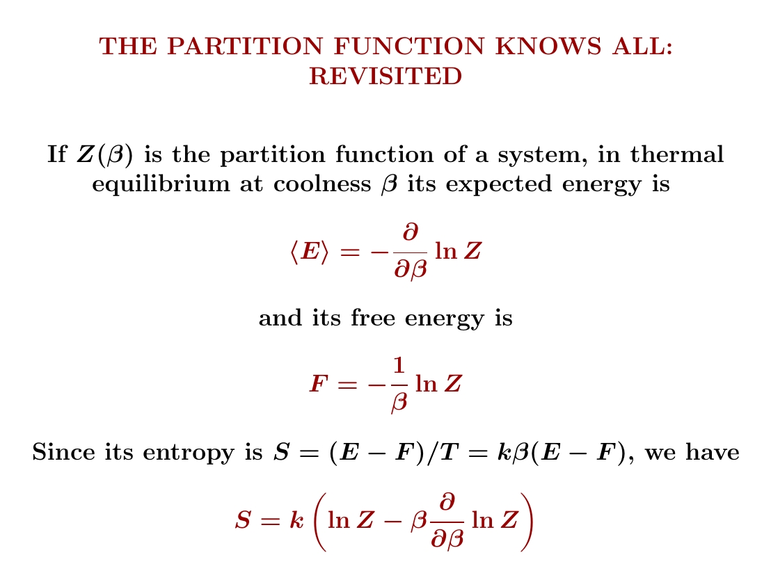
The partition function is all-powerful! If you know the partition function of a physical system, you can figure out its expected energy and entropy in thermal equilibrium! And more, too!
Let's see why.
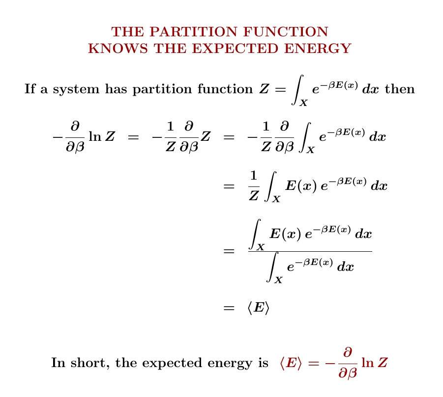
The expected energy \(\langle E \rangle\) is minus the derivative of \(\ln Z\) with respect to the coolness \(\beta = 1/kT\).
How do you show this? Easy: just take the derivative! You get a fraction, which is the expected value of \(E\) with respect to the Gibbs distribution.
The entropy is a bit more complicated. But don't be scared! Just let \(p(x)\) be the Gibbs distribution and work out its entropy \(-\int p(x) \ln p(x) dx\). Break the log of a fraction into two pieces. Then integrate each piece, and use what we just learned about \(\langle E \rangle \):
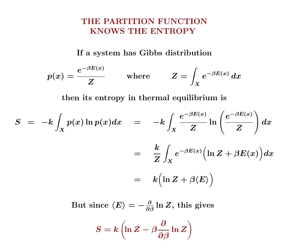
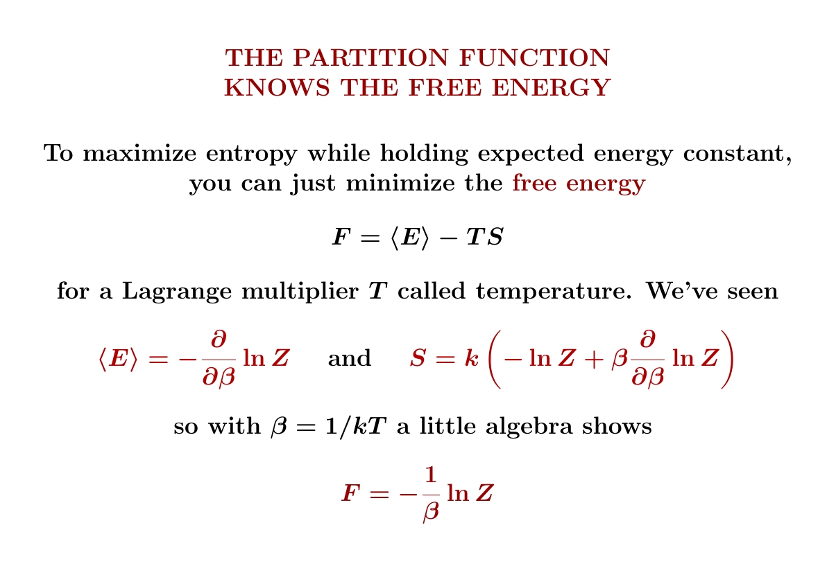
We can understand what's going on better if we bring in a concept I haven't mentioned yet: the 'free energy' $$ F = \langle E \rangle - TS $$ Since we know \(\langle E \rangle\) and \(S\), we can work out \(F\). And it's really simple! Much simpler than \(S\), for example. It's just \(-\frac{1}{\beta} \ln Z\).
In retrospect we can tell a simpler story, which is easier to remember.
The expected energy \(\langle E \rangle\) and free energy \(F\) are simple — and they look very similar! Entropy is their difference divided by \(T\), so it's more complicated.
But this was not the easy order to figure things out.
There's a huge amount to say about the free energy $$ F = \langle E \rangle - TS $$ or more precisely 'Helmholtz free energy', since there are other kinds. Roughly speaking, it measures the useful work obtainable from a system at a constant temperature!
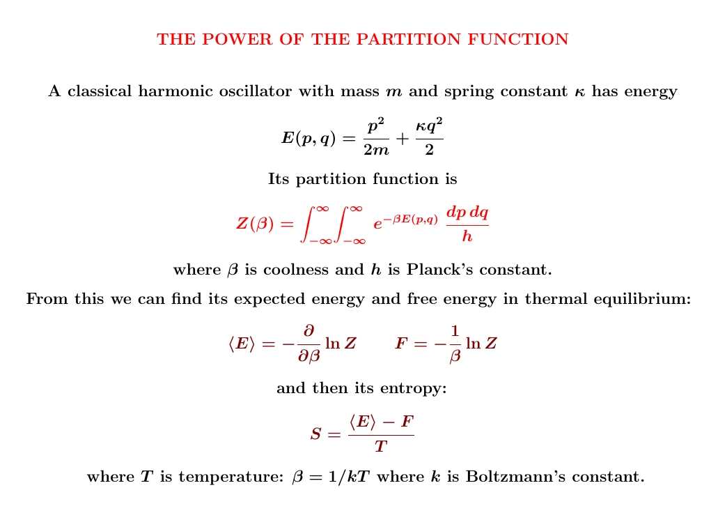
To test out the power of the partition function, let's use it to figure out the entropy of a classical harmonic oscillator.
We'll use it to compute the oscillator's expected energy and free energy. Then we just subtract those and divide by temperature!
In fact, I've already worked out the answer to this problem: $$ S = k \ln \left( \frac{kT}{\hbar \omega}\right) + k. $$ On September 9th I showed you how to compute the entropy up to an unknown constant by simple reasoning. You may enjoy recalling how that worked. Then on Steptember 10th I figured out the unknown constant, which gives the \(+k\) here. This required doing an ugly integral. Luckily it's enough to compute it in one example. I tried to make this look easy by a clever choice of units.
This approach led to some cool insights. But it was 'tricky', not systematic. The partition function method is systematic, so it's good for harder problems.
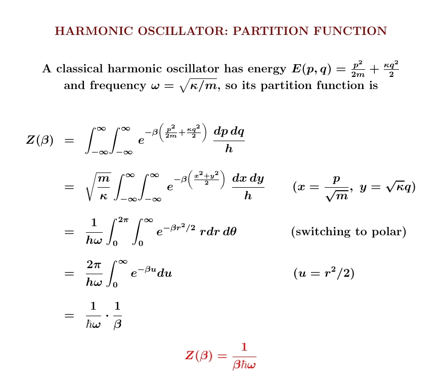
When we compute the entropy using a partition function, all the pain is concentrated at one point: computing the partition function!
For the harmonic oscillator, it's the integral of a Gaussian. A change of variables makes the Gaussian 'round', and then we use polar coordinates:
Once we know the partition function \(Z\) it's easy to compute the expected energy: just use $$ \langle E \rangle = - \frac{\partial}{\partial \beta} Z. $$ For the harmonic oscillator we already know the answer thanks to the equipartition theorem, which I proved on August 18th. But that's okay: this lets us check that we calculated \(Z\) correctly!
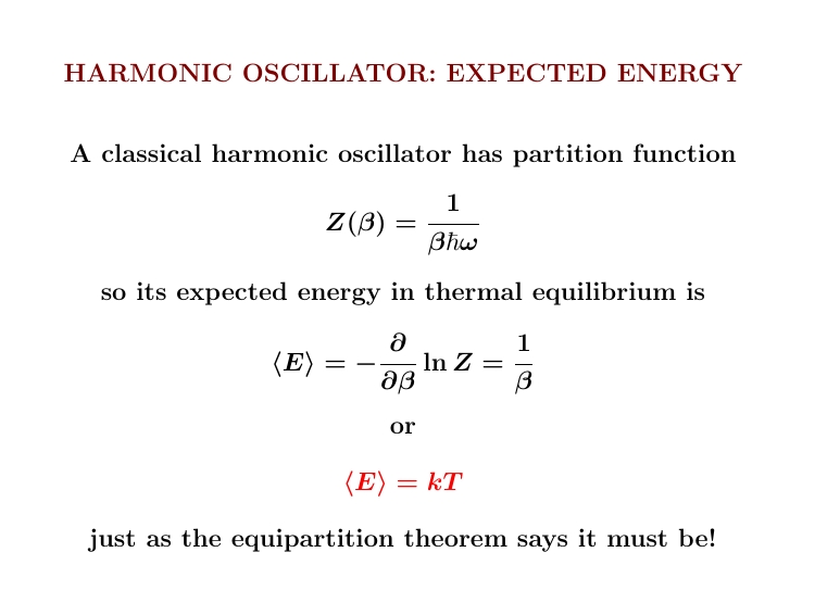
Remember, the equipartition theorem applies to a classical system whose energy is quadratic. If it has \(n\) degrees of freedom, then at temperature \(T\) it has $$ \langle E \rangle = \frac{n}{2} kT. $$ Our harmonic oscillator has n = 2, so we get \(\langle E \rangle = kT\). Good, that matches the partition function approach!
But the partition function lets us do more! It lets us compute the free energy, too, using $$ F = - \frac{1}{\beta} \ln Z $$ Unlike the expected energy, the free energy involves Planck's constant:

Note \(kT\) and \(\hbar \omega\) both have units of energy, so \(kT/\hbar \omega\) is dimensionless, which is good because we're taking its logarithm. Also note that the free energy is negative at high temperatures! That may seem weird, but it turns out to be good when we compute the entropy.
To compute the entropy, we just use $$ S = \frac{ \langle E \rangle - F}{T} $$ We get the answer we got before, of course:
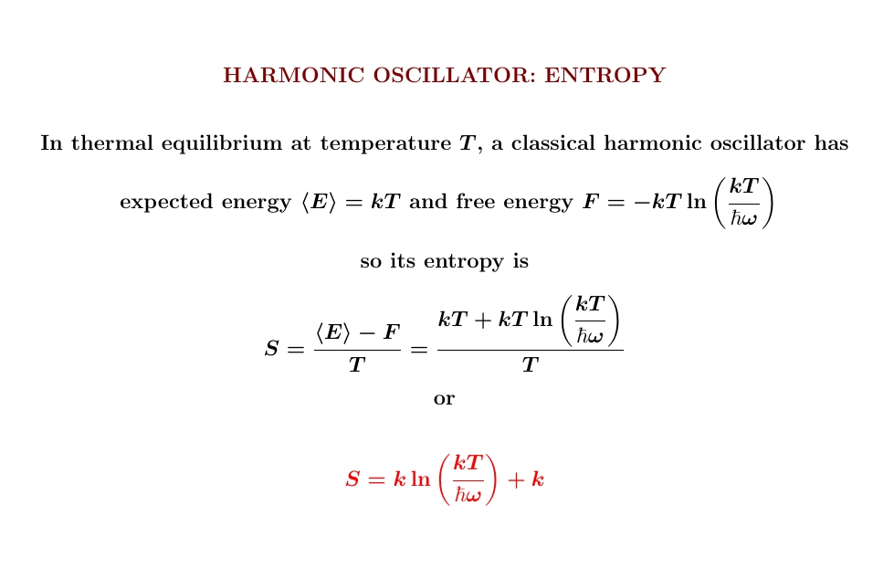
But now we get a new outlook on that 'mysterious constant' — the extra
\(+k\). Now we see it's the expected energy divided by \(T\). The
rest comes from free energy (which is subtracted).
September 26, 2022
Say you've got a set where each point has a number called its
'energy'. Then the partition function counts the points — but points
with large energy count for less! And the amount each point gets
counted depends on the temperature.

So, the partition function is a generalization of the 'cardinality' \(|X|\) - that is, the number of points of \(X\) - that works for sets \(X\) equipped with a function \(E\colon X \to \mathbb{R}\). It reduces to the cardinality in the high-temperature limit.
Just like the cardinality, the partition function adds when you take disjoint unions, and multiplies when you take products!
I need to explain this.
Let's call a set \(X\) with a function \(E \colon X \to \mathbb{R}\) an energetic set. I may just call it \(X\), and you need to remember it has this function. I'll call its partition function \(Z(X)\).
How does the partition function work for the disjoint union or product of energetic sets?
The disjoint union \(X+X'\) of energetic sets \(E\colon X \to \mathbb{R}\) and \(E' \colon X' \to \mathbb{R}\) is again an energetic set: for points in \(X\) we use the energy function \(E\), while for points in \(X'\) we use the function \(E'\). And we can show that $$ Z(X+X') = Z(X) + Z(X') $$ Just like cardinality!
The product \(X\ \times X'\) of energetic sets \(E\colon X \to \mathbb{R}\) and \(E' \colon X' \to \mathbb{R}\) is again an energetic set: define the energy of a point \((x,x') \in X \times X'\) to be \(E(x) + E(x')\). This is how it really works in physics. And we can show that $$ Z(X \times X') = Z(X)\, Z(X') $$ Just like cardinality!
If you like category theory, here are some fun things to do:
1) Make up a category of energetic sets.
2) Show the disjoint union of energetic sets is the coproduct in this category.
3) Show the cartesian product of energetic sets is not the product in this category.
4) Show that what I called the 'cartesian product' of energetic sets gives a symmetric monoidal structure on the category of energetic sets. So we should really write it as a tensor product \(X \otimes X'\), not \(X\times X'\).
5) Show this tensor product distributes over coproducts: \( X\otimes (Y+Z) \cong X\otimes Y + X\otimes Z\).
Last but not least:
6) Show that for finite energetic sets \(X\) and \(X'\), \(X \cong X'\) if and only if \(Z(X) = Z(X')\).
(Hint: use the Laplace transform.)
So, the partition function for finite energetic sets acts a lot like the cardinality of finite sets. It's a generalization of counting! And it reduces to counting as \(T \to +\infty\).
For the continuation of my course on entropy go to my October 2nd diary entry.
September 27, 2022
Why do quarks have charges 2/3 and -1/3? There's actually an
interesting theory about this. It was a lot of fun talking to Timothy
Nguyen about this sort of thing, starting from scratch and working out
the weird patterns in particle charges that hint at grand unified
theories.

Why does physics focus so much on position, velocity and acceleration — but not the higher time derivatives of position like jerk, snap, crackle and pop? There are many answers, starting with \(F = ma\). But I feel like explaining a fancy answer that's hard to find.
Start by assuming that we have a commutative algebra \(A\) of observables — an algebra over the real numbers, say. Also assume each observable \(a\in A\) generates a 1-parameter group of symmetries sending each observable \(b\in A\) to some observable \(b(t) \in A\) for each time \(t\in \mathbb{R}\). This idea is inspired by Noether's theorem, but we're making it into an axiom.
What does '1-parameter group' mean here? It means $$ b(0) = 0 $$ $$ b(s+t) = (b(s))(t) $$ for all \(s,t \in \mathbb{R}\), \(b \in A\).
What does 'symmetry' mean? For starters, we want these symmetries to be automorphisms of the algebra \(A\). This means that $$ (\alpha b)(t) = \alpha b(t) $$ $$ (b+c)(t) = b(t) + c(t) $$ $$ (bc)(t) = b(t) c(t) $$ for all \(\alpha \in \mathbb{R}\), \(b,c\in A\).
Now let's cast rigor to the wind and assume everything is differentiable and we can do all the formal manipulations we want. We could make things rigorous using more analysis, and more assumptions, but let's not. Let's define a bracket operation on \(A\) by $$ \{a,b\} = \left. \frac{d}{dt} b(t) \right|_{t = 0} $$ If we cast rigor to the wind, differentiate the three equations above and set \(t = 0\) we get $$ \begin{array}{cclc} \{a , \alpha b\} &=& \alpha \{a,b\} & \qquad (1) \\ \{a, b+c \} &=& \{a,b\} + \{a,c\} & \qquad (2) \\ \{a, bc \} &=& \{a,b\} c + b\{a,c\} & \qquad (3) \end{array} $$ Mathematicians summarize these by saying that the operation \( \{a,-\}\) is a derivation of \(A\).
Next, let's assume our one-parameter group preserves the operations \(\{-,-\}\). After all, the 'symmetries' generated by our observables should be symmetries of the whole setup here! So, we expect $$ \{b(t), c(t)\} = \{b,c\}(t) $$ for all \(b,c \in A\). If we differentiate this and set \(t = 0\), we get: $$ \{a,\{b,c\}\} = \{\{a,b\},c\} + \{b,\{a,c\}\} \quad \; (4) $$ The Jacobi identity!
Next, assume any observable generates symmetries that preserve itself: $$ a(t) = a $$ For example time evolution conserves energy, translation preserves momentum, etc. Differentiating this equation, we expect $$ \qquad \quad \{a,a\} = 0 \qquad \qquad \qquad \qquad (5) $$ Using this together with equations (1) and (2) we can prove that $$ \{a,b\} = -\{b,a\} $$ So, our bracket makes \(A\) into a Lie algebra. Then equation (3) says that \(A\) is a Poisson algebra.
In short: from the idea that observables form a commutative algebra, with each one generating symmetries that preserve the whole setup — including the way observables generate symmetries! — we are led to expect that observables form a Poisson algebra. And if the details of analysis work out, we get an abstract version of Hamilton's equations: $$ \frac{d}{dt} b(t) = \{a,b(t)\} $$ Next, assume that as a commutative algebra, \(A\) is the algebra of smooth functions on some manifold \(X\). Points in \(X\) are states of our physical system.
Then because \(A\) is a Poisson algebra, \(X\) becomes a Poisson manifold.
Now any derivation \(\{a,-\}\) comes from a smooth vector field on \(X\). And if \(X\) is compact, all the annoying bits of analysis that I sidestepped actually do work, because every smooth vector field gives a 1-parameter group of diffeomorphisms of \(X\), and vice versa!
But where did position and velocity go in all this? Everything so far is very general.
Here's the deal: the nicest Poisson manifolds are the symplectic manifolds, which can be covered by charts where the coordinates stand for position and momentum!
The existence of these charts is guaranteed by Darboux's theorem. And in these coordinates, the abstract Hamilton's equations I wrote: $$ \frac{d}{dt} b(t) = \{a,b(t)\} $$ become the usual Hamilton's equations describing the first time derivatives of position and momentum!
Now, it looks like there's a gap in my story leading from general abstract nonsense to the familiar math of position and momentum: not every Poisson manifold is symplectic. But lo and behold, every Poisson manifold is foliated by symplectic leaves.
Yes: every point of a Poisson manifold lies on an immersed submanifold with a symplectic structure, called a 'symplectic leaf'. And if you solve Hamilton's equations with any Hamiltonian, a point that starts on some leaf will stay on that leaf!
So while there are still some rough edges in this story, physicists
can almost go straight from a commutative algebra where each
observable generates symmetries preserving that observable, to the
equations for the time derivatives of momentum and position!
September 29, 2022
What the heck is an ultrafilter? You can think of it as a
'generalized element' of a set — like how \(+\infty\) and
\(-\infty\) are not real numbers, but sometimes we kind of act like
they are. We just need to make up rules that these generalized
elements should obey!
If we have a set \(X\), all a generalized element does is tell us whether it's "in" any subset \(S \subseteq X\). Here "in" is in quotes, because a generalized element may not be an actual element of \(X\). If it is, "in" just means the usual thing. But otherwise, not.
For example, we'll say +∞ is "in" a subset \(S \subseteq \mathbb{R}\) if and only \(\S\) contains all numbers \(\ge c\) for some \(c \in \mathbb{R}\). We're not saying \(+\infty\) is actually in \(S\). It's just a generalized element. This example will help you understand the rules!
So, if \(x\) is a generalized element of a set \(X\), what rules must it obey? Here they are:
Puzzle. Show that if \(X\) is finite, all its generalized elements come from actual elements.
So, generalized elements are only interesting when X is infinite.
But I lied!
Suppose \(+\infty\) is "in" a subset \(S \subseteq \mathbb{R}\) if and only \(\S\) contains all numbers \(\ge c\) for some \(c \in \mathbb{R}\). Then this does not define a generalized element, because one of rules 1)-4) does not hold! Which one?
In fact — and this is the tragic part — it's basically impossible to concretely describe any generalized elements of an infinite set, except for actual elements! So, I cannot show you any interesting examples.
The problem is that by rule 4) we need to decide, for each \(S \subseteq X\), whether our generalized element is "in" \(S\) or "in" its complement. That's a lot of decisions! And we need to make them in a way that's consistent with rules 1)-3).
Except for actual elements, nobody can do it!
So, people resort to the Axiom of Choice. This is an axiom of set theory specially invented to deal with situations where you have too many decisions to make, and no specific rule for making them. You point to the genie called Axiom of Choice and say "he'll do it".
If you're willing to accept the Axiom of Choice, generalized elements — usually called 'ultrafilters' — are an amazingly powerful tool. I've shied away from them, because I have trouble understanding a subject without concrete examples. But they're still interesting!
For more on ultrafilters try these:
Yesterday I defined ultrafilters on a set \(X\), which I likened to 'generalized elements' of \(X\). Let \(\beta X\) be the set of ultrafilters on a set \(X\). Every element of \(X\) gives a generalized element, so we get a natural map $$ i \colon X \to \beta X $$ Anything you do in math, that's fun, you should try doing again. So, what about 'generalized generalized elements'? They make sense — they are elements of \(\beta\beta X\) — but they can always be turned into generalized elements! Yes, there's a natural map $$ m \colon \beta\beta X \to \beta X $$ Now, this should remind you of how we can take the set of lists of elements of a set \(X\) — call it \(LX\) — and get natural maps $$ i \colon X \to LX $$ sending an element to its one-item list, and $$ m \colon LLX \to LX $$ flattening a list of lists to a list. Indeed, we can use \( m \colon LLX \to LX \) to define two ways to flatten a list of lists of lists to a list, but they turn out to be equal!
Similarly our maps \(m \colon \beta\beta X \to \beta X\) give two ways to turn a generalized generalized generalized element into a generalized element, but they're equal!
This is called the 'associative law' for \(m \colon \beta\beta X \to \beta X\).
The maps \(m\) and \(i \colon X \to \beta X\) also obey two 'unit laws', which say that two ways to turn a generalized element into a generalized generalized element and then back into a generalized element get you back where you started.
To summarize all this, we say that ultrafilters, just like lists, give a 'monad' on the category of sets: $$ \beta \colon \mathrm{Set} \to \mathrm{Set} $$ There are lots of fun things to do with monads, which show up a lot in math and computer science, so let's try some with \(\beta\)!
We can talk about 'algebras' of a monad. An algebra of the list monad \(L\) is a set \(X\) together with a map $$ a \colon LX \to X $$ obeying some rules explained below. It winds up being a monoid, where you can multiply a list of elements and get one element!
Similarly, an algebra of the ultrafilter monad is a set \(X\) together with a map $$ a \colon \beta X \to X $$ obeying the same rules. So, it's a set where you know how to turn any generalized element into an actual element in some very well-behaved way. Can you guess what it is?
An algebra of the ultrafilter monad is the same as a compact Hausdorff space!
It's as if topology appears out of thin air! The proof of this wonderful result is sketched here:
and it seems to be due to Ernest Manes, maybe in 1976.If you know enough stuff about how ultrafilters show up in topology, you may not agree that compact Hausdorff spaces appear 'out of thin air' here But the ultrafilter monad really does come from very pure ideas: it's the right Kan extension of the inclusion $$ \mathrm{FinSet} \to \mathrm{Set} $$ along itself. Read this for more:
So, the interplay between finite sets and sets gives the ultrafilter monad and then compact Hausdorff spaces! These spaces are 'sets equipped with a structure that makes them act almost finite' — in that every generalized element gives an element.
Condensed or pyknotic mathematics is a new twist on these ideas. There are many points of view on this, but one is that we can use the relation between two ways of describing algebraic gadgets — monads and Lawvere theories — and then run completely wild!
Take the category of 'finitely generated free' algebras of a monad \(T \colon \mathrm{Set} \to \mathrm{Set}\): namely, those of the form \(TX\) for finite sets \(X\). The opposite of this category is a Lawvere theory \(L\).
\(L\) knows all the finitary operations described by our monad T — but only those! They become the morphisms of \(L\).
Now, the ultrafilter monad \(\beta \colon \mathrm{Set} \to \mathrm{Set}\) is insanely nonfinitary. In fact it has operations whose arities are arbitrarily large cardinals! So let's take the category of all free algebras of \(\beta\) and form its opposite, \(L\). This is like a monstrously large Lawvere theory.
Then, we can define a 'pyknotic set' to be a finite-product-preserving functor $$ F \colon L \to \mathrm{Set} $$ There are some size issues here, since as I've described it \(L\) is a proper class. Barwick & Haine handle these carefully using the axiom of universes — read this introduction for more:
But the weird (and important) part is that we're only requiring our pyknotic set \(F\) to preserve finite products! If it preserved all products, I'd expect it to be the same as an algebra of the ultrafilter monad: that is, a compact Hausdorff space.
Indeed, compact Hausdorff spaces give pyknotic sets. So do topological space of many other kinds! But the really interesting pyknotic sets are the new ones, that aren't topological spaces.
For example, \(\mathbb{R}\) with its usual topology is a 'pyknotic group': a group in the category of pyknotic sets. So is \(\mathbb{R}\) with its discrete topology. The quotient of the former by the latter is a pyknotic group with one element.... but a nontrivial pyknotic structure!