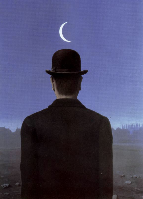
One great thing about Magritte's painting The Schoolmaster is
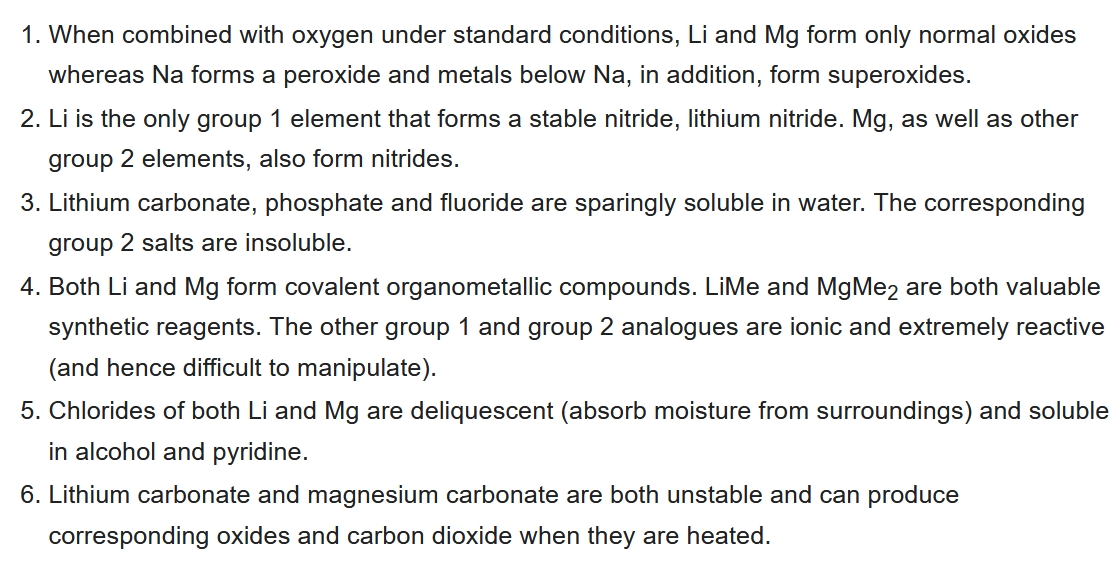
that while surreal, it depicts a scene that could be perfectly real.
December 2, 2021
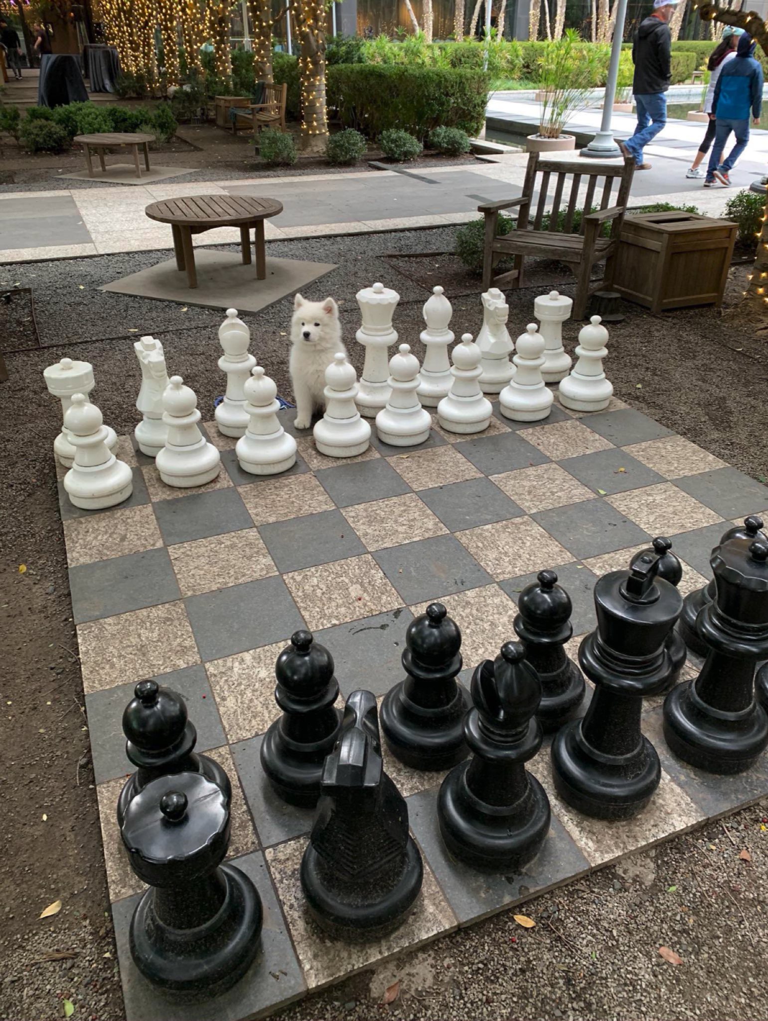
Sometimes you just try to blend in and hope nobody notices.
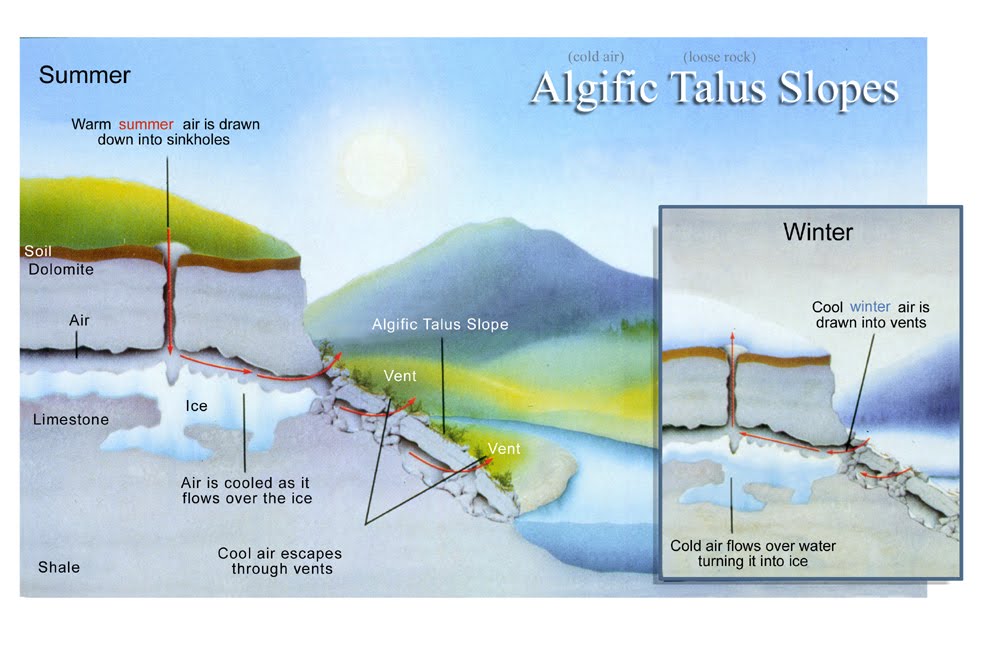
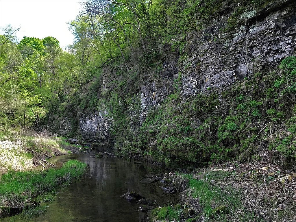
These unusual ecosystems are called algific talus slopes, where 'algific' means 'cold producing' and 'talus' refers to the piles of broken rock near the base of a cliff. They are mostly found in the Driftless Area, a region in Minnesota, Wisconsin, Illinois, and especially Iowa that for some unknown reason was never hit by glaciers during the last ice age. Elsewhere, glaciers crushed the hills and caves. There are also a few algific talus slopes in the Allegheny Mountains of West Virginia.
For a bit more on this fascinating subject, read these:
The vegetative community on algific talus slopes is different than the surrounding forest and typically contains ferns, mosses, liverworts, evergreen species such as Canada yew and balsam fir, birch, basswood, and sugar maple, and boreal disjunct herbs and ferns.
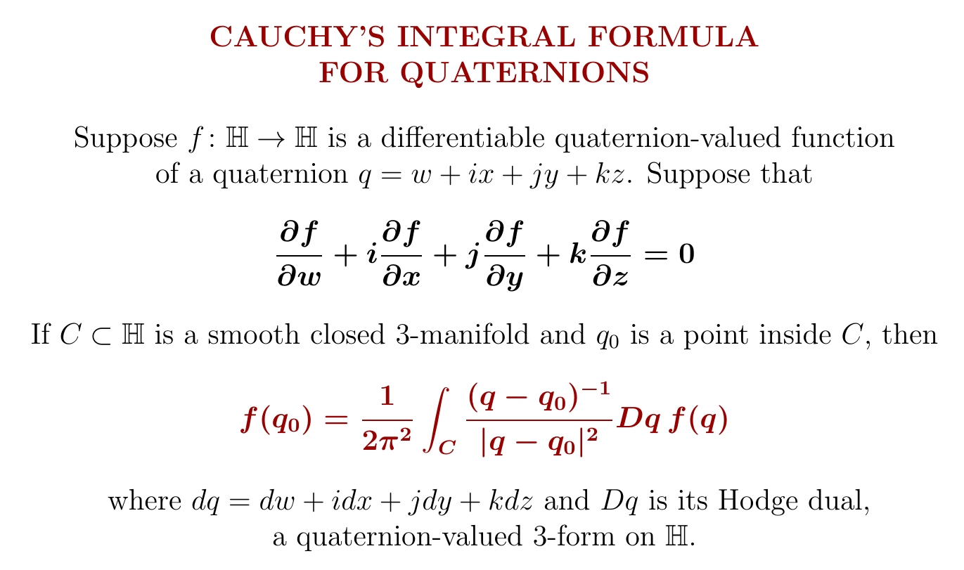
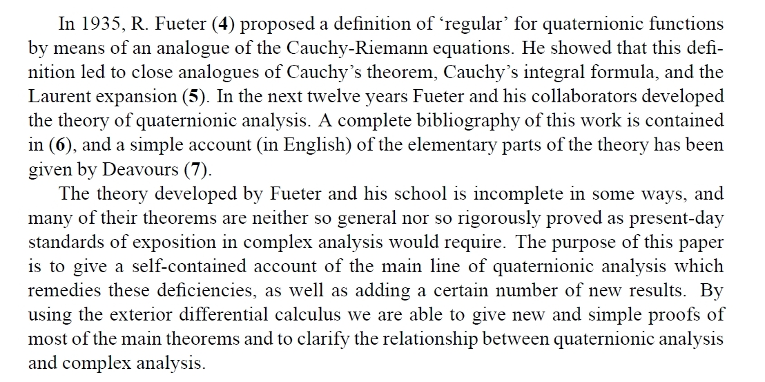
If you've met Cauchy's integral formula in complex analysis, guess what: there's a version for the quaternions too! It works for any function that obeys the quaternionic version of the Cauchy–Riemann equation $$ \frac{\partial f}{\partial x} + i \frac{\partial f}{\partial y} = 0 $$ It was discovered by Rudolf Fueter in 1936.
Quaternionic analysis isn't quite as beautiful as complex analysis, mainly because if you multiply two solutions of $$ \frac{\partial f}{\partial w} + i \frac{\partial f}{\partial x} + j \frac{\partial f}{\partial y} + k \frac{\partial f}{\partial z} = 0 $$ you don't get another solution! But it ain't chopped liver, neither. It deserves a little love.
There's a lot of confusing literature on quaternionic analysis. This is good:
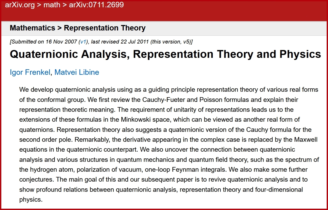
Here's another good paper, more advanced:
It shows some really deep math, connected to physics, comes out of quaternionic analysis!
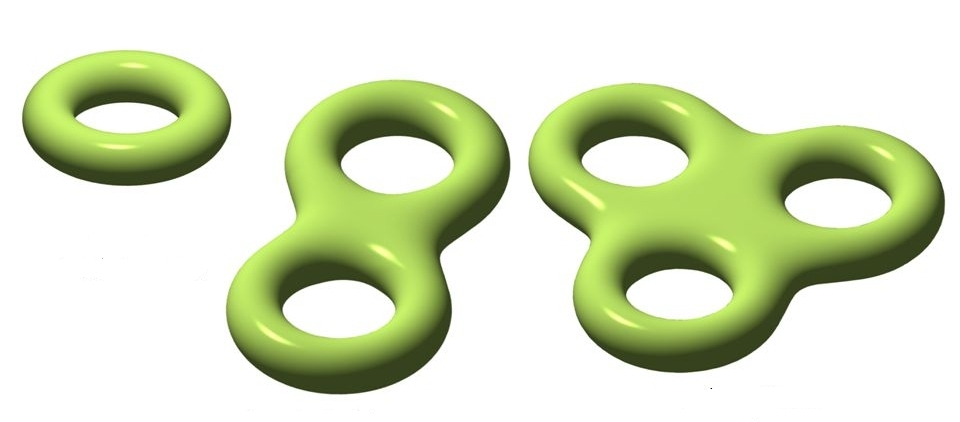
The surface of a doughnut is called the 'boundary' of the doughnut. Indeed any compact oriented 2-manifold, like these here, can be filled in — it's the boundary of some compact oriented 3-manifold. The same thing is true one dimension up — but not two dimensions up!
(I say 'oriented' because the real projective plane \(\mathbb{R}\mathrm{P}^1\) is a compact 2-manifold that's not orientable, and it's not the boundary of any compact 3-manifold. There are also good reasons to stick with compact manifolds.)
The boundary of a manifold has no boundary itself: if \(\partial M\) is the boundary of the manifold \(M\) then $$ \partial \partial M \cong \emptyset $$ So here's the 2d story again, more precisely: every compact orientable 2-manifold \(M\) with no boundary is the boundary of some compact orientable 3-manifold. In symbols: if \(\partial M = \emptyset\) then there's an \(N\) with \(\partial N = M\).
The story one dimension up is just the same, but harder to see: every compact orientable 3-manifold with no boundary is the boundary of some compact orientable 4-manifold.
But this pattern breaks down when we go up another dimension! The culprit is called \(\mathbb{C}\mathrm{P}^2\).
\(\mathbb{C}\mathrm{P}^2\), the 'complex projective plane', is the set of all 1d subspaces of \(\mathbb{C}^3\). \(\mathbb{C}\mathrm{P}^2\) is a compact orientable 4-manifold, and it has no boundary... but it's not the boundary of any compact orientable 5-manifold!
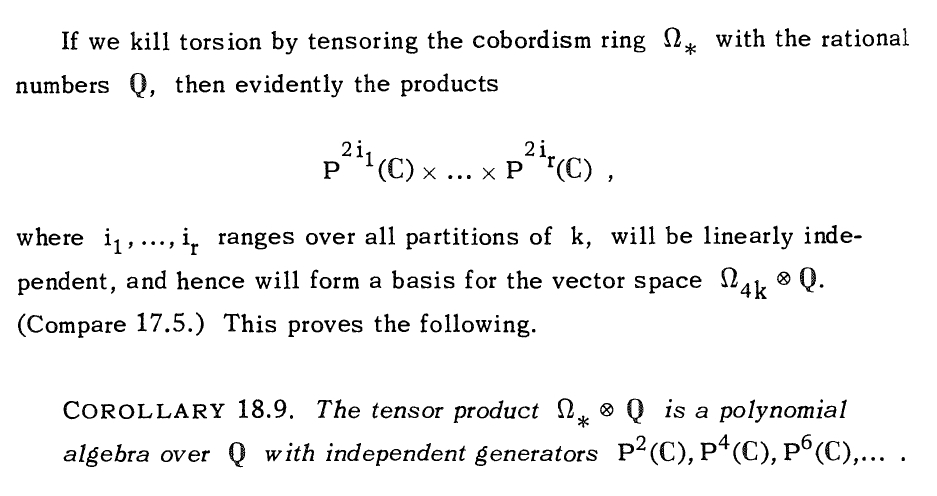
This is the beginning of a bigger story! The boundary \(\partial\) also obeys $$ \partial(M + N) \cong \partial M + \partial N $$ $$ \partial (M \times N) \cong \partial M \times N + M \times \partial N $$ where \(+\) means disjoint union and \(\times\) means cartesian product. So, we can take linear combinations of compact oriented manifolds with \(\partial M = \emptyset\), and mod out by those that are boundaries, and get a ring!
If we take linear combinations using the rational numbers, this we get the algebra of polynomials in countably many variables, which stand for \(\mathbb{C}\mathrm{P}^2, \mathbb{C}\mathrm{P}^4, \mathbb{C}\mathrm{P}^6, \dots \). Here \(\mathbb{C}\mathrm{P}^n\), 'complex projective \(n\)-space', is the set of 1-dimensional subspaces of \(\mathbb{C}^{n+1}\). This is a compact oriented manifold of dimension \(2n\).
So, working over the rational numbers, we can completely understand this stuff!
For example, \(\mathbb{C}\mathrm{P}^2, \mathbb{C}\mathrm{P}^4, \mathbb{C}\mathrm{P}^6,\) etc. have dimensions that are multiples of \(4\). So, whenever \(n\) is a multiple of \(4\), there are compact oriented \(n\)-dimensional manifolds that have no boundary, but aren't themselves boundaries of compact oriented manifolds!
But working with rational linear combinations waters things down! Using this trick we can't see that even though \(5\) isn't a multiple of \(4\), there's a compact oriented \(5\)-manifold without boundary that's not the boundary of some compact oriented \(6\)-manifold!
This 5-manifold \(W\) is called the 'Wu manifold', and $$ W = \mathrm{SU}(3)/\mathrm{SO}(3) $$ Even though \(W\) is not a boundary, \(W + W\) is! And when we work with rational linear combinations we can divide by 2, so \(W + W = 0\) implies \(W = 0\) in the ring I described.
To detect these subtler phenomena, we should take integer linear combinations of compact oriented manifolds without boundary, mod boundaries. This gives a ring called the oriented cobordism ring, \(\Omega^{\mathrm{SO}}\).
This ring is pretty well understood:
![]()
The structure of matter is a great game of Go, played with electrons. You can't put two in the same square.
This shows how many electrons you can easily remove from transition metals. For iron, Fe: 2, 3, 4 (harder), 5 or 6 (harder).
Remember from my November 30th entry: the math of polynomials creates
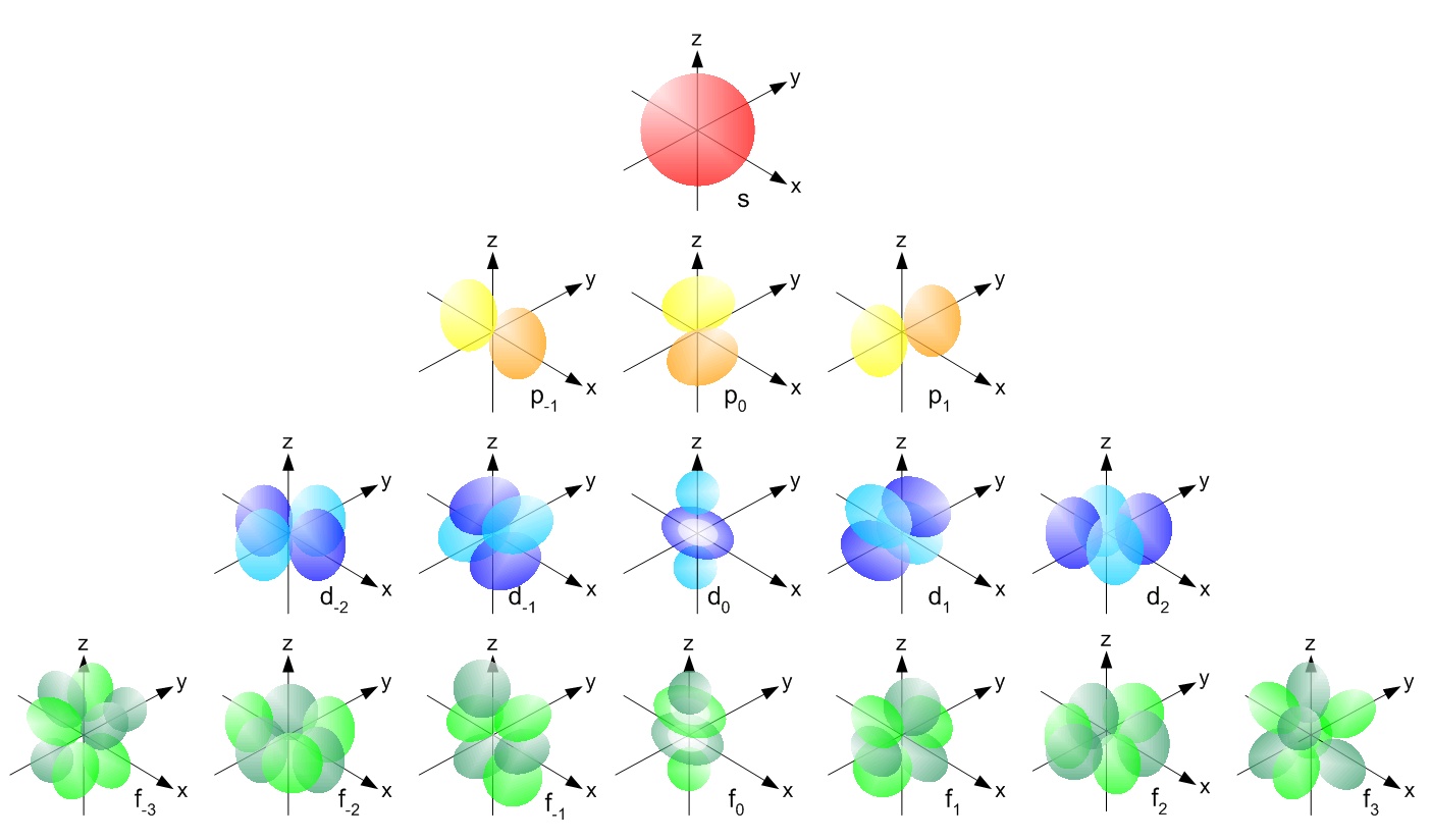
The transition metals use the d orbitals for their outermost electrons. This is why there are 10 transition metals per row!
Look, here they are: 10 per row, all because there's a 5d space of quadratic polynomials in \(x,y,z\) with vanishing Laplacian! Math becomes matter.
Some of these d orbital electrons are easily removed. So the transition metals conduct electricity!
Also, in different 'oxidation states', like in solutions, they lose different numbers of electrons.
For example, scandium has all the electrons of argon (Ar) plus two in an s orbital and one in a d orbital. It can lose 3 electrons. Titanium has one more electron, so it can lose 4. And so on.
That accounts for the most obvious pattern in the chart below: the diagonal lines sloping up. But everything is complicated because electrons interact! So the trend doesn't go on forever: iron (Fe) does not easily give up 8 electrons. And there's more going on, too.
(If you look carefully you'll see the two charts above don't completely agree: the chart in color includes some quite rare oxidation states.)
You can calculate exactly how all this stuff works by doing computations with Schrödinger's equation — or the Dirac equation, which takes special relativity into account, more important for heavy elements.
But there are many simple patterns you can understand more easily! Chemistry is a fascinating mix of math and rules of thumb. For more, see:
I'll be so glad when this is finally up and running. There's still
plenty that can go wrong between now and then, since they need to cut
a trench in the rocky hill in our back yard, and through the retaining
wall at the bottom of that hill.
December 10, 2021
I posted some blog articles about the math of the periodic table,
based on my explanations here:
The second heaviest: tennessine.
Combine them and you get oganesson tetratennesside, OgTs4 — so heavy that special relativity makes it weird!
Alas, it decays radioactively in less than a millisecond.
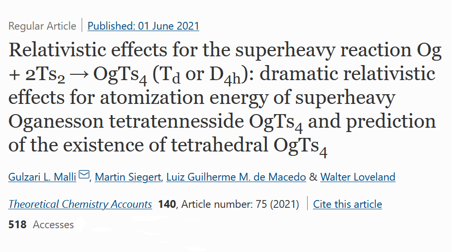
Work on oganesson tetratennesside is purely theoretical, since both elements are artificially made in tiny amounts, and short-lived. The half-life of tennessine is at most 51 milliseconds, while for oganesson it's just 0.69 milliseconds! But we can study the compounds they make using computer calculations. And it seems OgTs4 should be possible.
I said "noble gas", but oganesson should actually be a noble solid with a melting point of roughly 50 Celsius, due to the effects of relativity on its fast-moving electrons. And it should be much more reactive than xenon or radon!
Tennessine is a halogen, in the same column of the periodic table as fluorine, chlorine, bromine, iodine and astatine. These get less reactive as we move down the column.
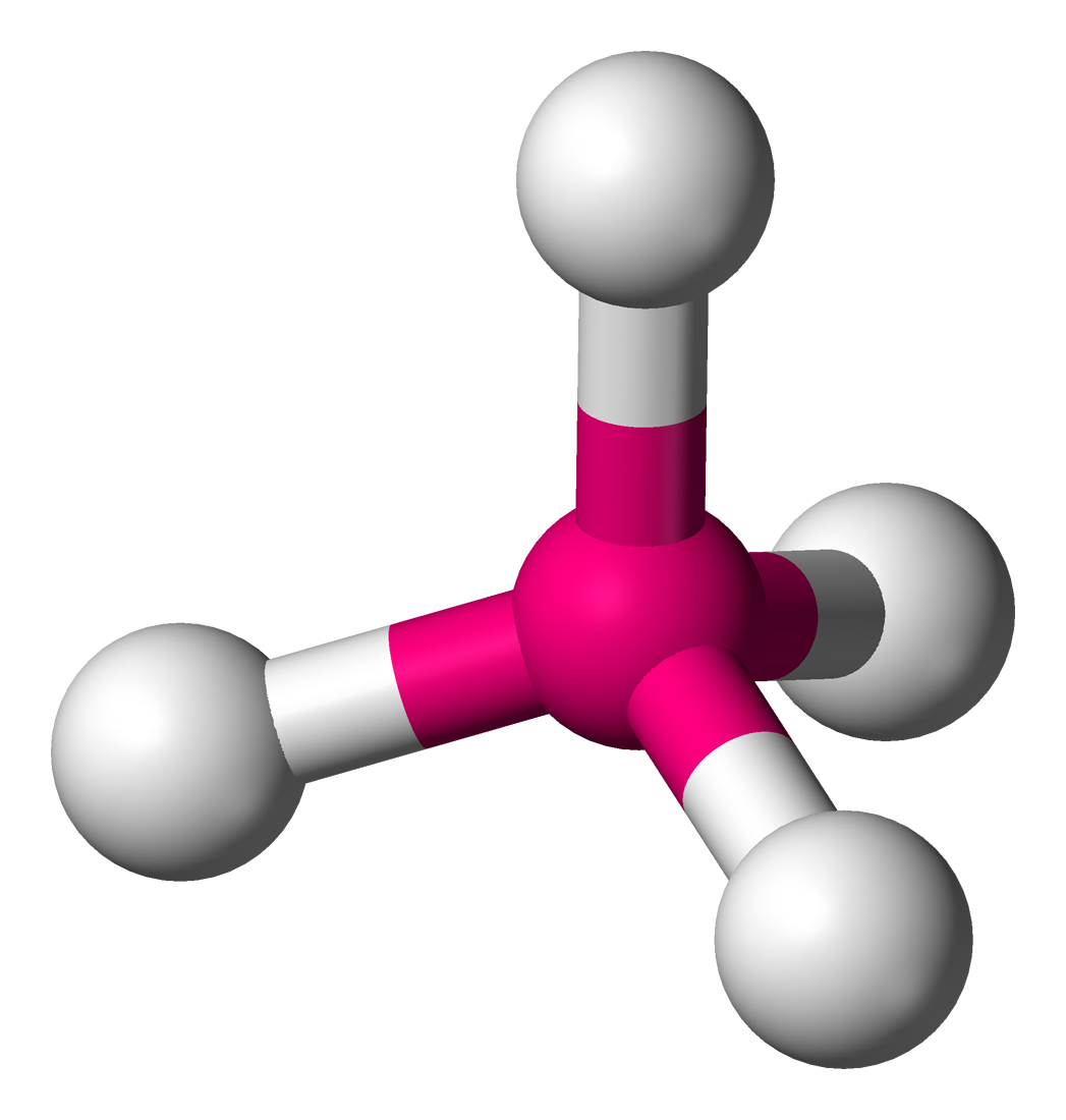
Fluorine is so aggressive that xenon tetrafluoride exists! This molecule is flat.
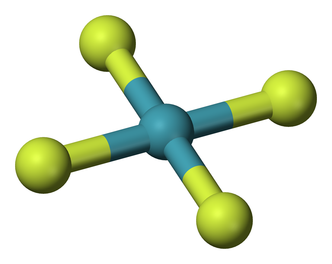
With 586 electrons, OgTs4 must be a nightmare to compute. This paper studies it using the Dirac–Fock method, a version of Hartree–Fock that takes special relativity into account. It claims OgTs4 should be tetrahedral, not flat, due to these effects!
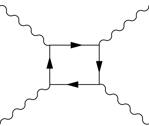
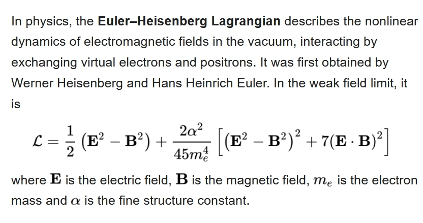
Light can bounce off light by exchanging virtual charged particles! This makes Maxwell's equations nonlinear, even in the vacuum — but only noticeably so when the electric field is \(10^{18}\) volts/meter or more. This is an enormous electric field, able to accelerate a proton from rest to Large Hadron Collider energies in just 5 micrometers!
In 2017, light-on-light scattering was seen at the LHC when they shot lead ions past each other:
Direct evidence for light-by-light scattering at high energy had proven elusive for decades, until the Large Hadron Collider (LHC) began its second data-taking period (Run 2). Collisions of lead ions in the LHC provide a uniquely clean environment to study light-by-light scattering. Bunches of lead ions that are accelerated to very high energy are surrounded by an enormous flux of photons. Indeed, the coherent action from the large number of 82 protons in a lead atom with all the electrons stripped off (as is the case for the lead ions in the LHC) give rise to an electromagnetic field of up to \(10^{25}\) volts per metre. When two lead ions pass close by each other at the centre of the ATLAS detector, but at a distance greater than twice the lead ion radius, those photons can still interact and scatter off one another without any further interaction between the lead ions, as the reach of the (much stronger) strong force is bound to the radius of a single proton. These interactions are known as ultra-peripheral collisions.
But now people want to see photon-photon scattering by shooting lasers at each other! One place they'll try this is at the Extreme Light Infrastructure.
In 2019, a laser at the Extreme Light Infrastructure in Romania achieved a power of 10 petawatts for brief pulses — listen to the announcement for what means!
I think it reached an intensity of \(10^{29}\) watts per square meter, but I'm not sure. If you know the intensity \(I\) in watts/square meter, for a plane wave of light you can compute the maximum strength \(E\) of the electric field (in volts/meter) by $$ I = \frac{1}{2} \varepsilon_0 c E^2 $$ where \(\varepsilon_0\) is the permittivity of the vacuum and \(c\) is the speed of light. According to Dominik Wild, \(I = 10^{29}\) watts per square meter gives \(E \approx 10^{16}\) volts/meter. If so, this is 1/100 the field strength needed to see strong nonlinear corrections to Maxwell's equations.
In China, the Station of Extreme Light plans to build a laser that makes brief pulses of 100 petawatts. That's 10,000 times the power of all the world’s electrical grids combined! They're aiming for an intensity of \(10^{28}\) watts/square meter:
The modification of Maxwell's equations due to virtual particles was worked out by Heisenberg and Euler in 1936. (No, not that Euler.) They're easiest to describe using a Lagrangian, but if we wrote out the equations we'd get Maxwell's equations plus extra terms that are cubic in \(\mathbf{E}\) and \(\mathbf{B}\).
For more, read these:

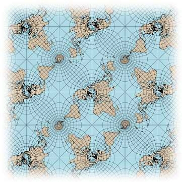
The philosopher Peirce worked at the U. S. Coast and Geodetic Survey, and in 1876 he invented this map. It's a way of wrapping a plane around a sphere while preserving angles — except at four points. This is an 'elliptic function'.
In general you get an 'elliptic function' by taking the plane and mapping it to the sphere in a way that's periodic in two directions, and angle-preserving at as many points as possible. It can't be angle-preserving everywhere: failing at 4 points of the sphere is the best you can do.
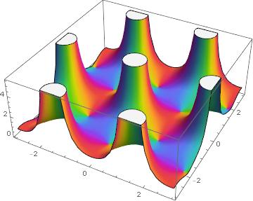
The most famous is the Weierstrass elliptic function. Here's a picture of it where different points of the sphere are indicated with different colors, hue indicating longitude and brightness latitude:
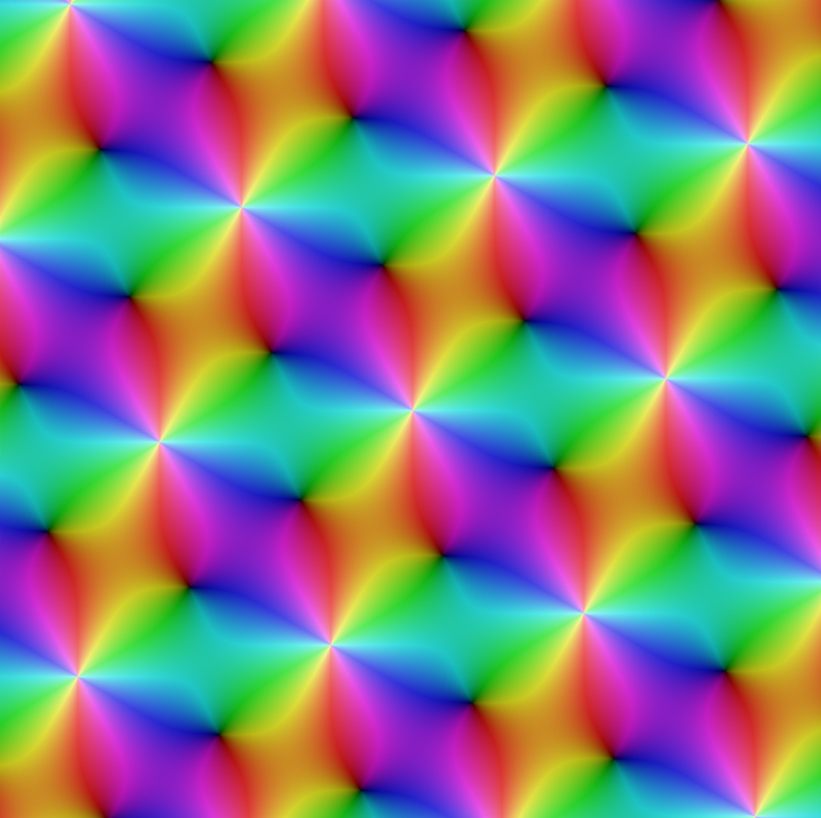
We can think of the plane as the complex plane, and the sphere as the Riemann sphere: the complex plane plus one point, \(\infty\). Then can get an elliptic function by adding up an infinite series of complex functions, each of which equals \(\infty\) at just one point, where these points form a lattice in the plane. Here's how it looks when you start adding more and more of those functions:

You can read more about Peirce's map and its connection to elliptic functions here:
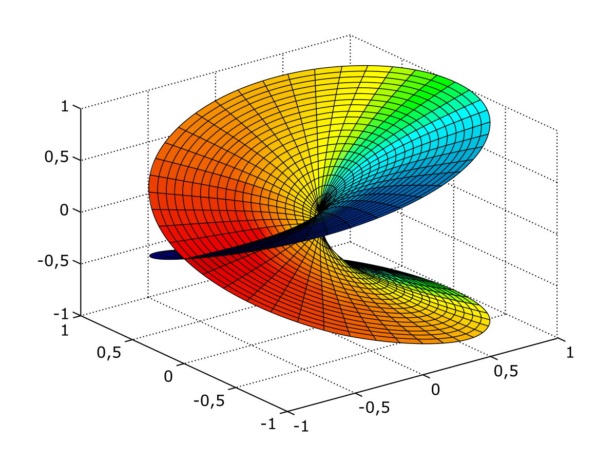
There are 2 points on the colored surface over each point in the plane below — except right in the middle, where there's just one. So we say the map from the colored surface to the plane below has a "branch point of ramification index 2".
The Riemann–Hurwitz formula relates the topology of two surfaces to the ramification indices of a map between them. I'll state it a bit loosely here, so you can quickly get the idea:

To understand it, let's look at a couple of examples.
You can wrap the sphere around itself \(n\) times using a map that's \(n\)-1 except at the north and south poles, which are branch points of ramification index \(n\). Here \(\chi(S) = \chi(S') = 2\) since \(S = S'\), the sphere, has no holes. So Riemann–Hurwitz says $$ 2 = n \times 2 - (n-1) - (n-1) $$ An 'elliptic function' is a kind of map from the torus to the sphere. This map is 2-1 except at 4 points, which are branch points of ramification index 2. You can see two of the branch points in this picture by Greg Egan. The other two are behind the picture.
For an elliptic function \(\chi(S) = 0\) and \(\chi(S') = 2\), since
the torus \(S\) has one hole and the sphere \(S'\) has none. Since this
function is 2-to-1 except for 4 points of ramification index 2,
Riemann–Hurwitz says
$$ 0 = 2 \times 2 - 4 \times (2 - 1) $$
December 15, 2021
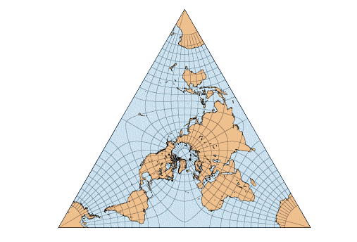
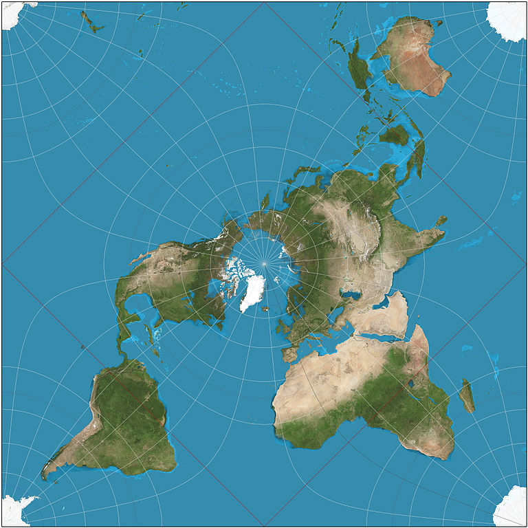
You can map the torus to the sphere in a way that's 2-1 except for 4 points where it's 1-1, called 'branch points'. If you put these 4 points at the vertices of a regular tetrahedron, you get the above map of the Earth.
Wait, how do you get a map of the Earth?
First you map the torus to the sphere — the Earth — in a 2-1 and angle-preserving way except for branched points at the vertices of a tetrahedron. Then you unroll the torus and get a parallelogram.
Then cut that parallelogram in half and you're done!
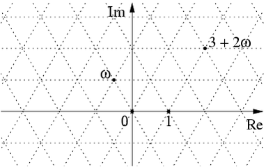
Your parallelogram, you see, will consist of 2 equilateral triangles stuck together, as shown here. And hiding behind this trick are the Eisenstein integers: the complex numbers \(a + b \omega\) where \(a,b\) are integers and \(\omega\) is a nontrivial cube root of 1.
The Eisenstein integers are closed under addition and multiplication! So are the Gaussian integers, \(a+bi\) where \(a\) and \(b\) are integers. These are a bit less exciting, but we can also use these to build a branched double cover of the sphere by the torus.
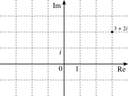
So the Gaussian integers also give a map of the Earth! I mentioned this one a while back — it was discovered by the philosopher C. S. Peirce.
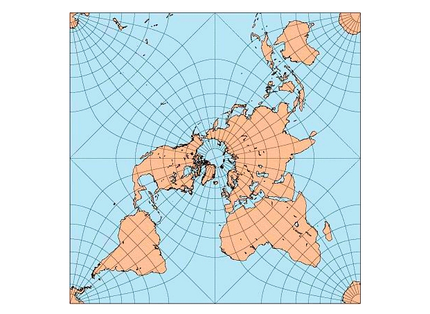
And now it's time to come clean: a map the torus to the sphere that's 2-1 and angle-preserving except at 4 points where it's 1-1 is usually called an elliptic function on an elliptic curve. I've just shown you the two most symmetrical ones! And as we saw yesterday, the number 4 is no accident here: it's forced on us by the Riemann–Hurwitz theorem.
There's lots more to say, but not today!
The nice maps were drawn by Carlos Furuti... but his website seems to be defunct, so take a look at the version on the WayBack Machine:
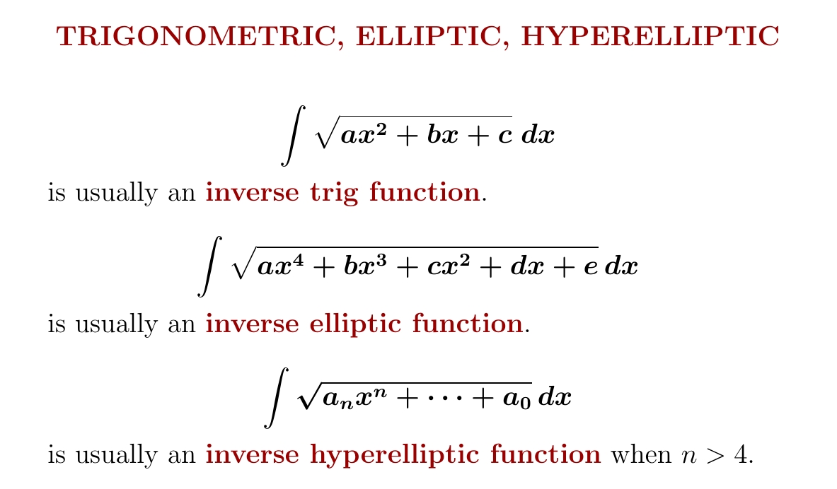
In the 1800s any really good mathematician would know about elliptic functions: they're the next thing after trig functions. Now as a species we know lots more about them — but a smaller fraction of mathematicians know about them.
And then come hyperelliptic functions!
Geometrically, an elliptic function defines a two-fold branched cover of the Riemann sphere by a torus. An example is shown below by Greg Egan. Similarly, a hyperelliptic function defines a two-fold branched cover of the Riemann sphere by an \(n\)-holed torus with \(n > 1\).
No matter how we make a torus into a Riemann surface, we can use it to get a two-fold branched cover of the Riemann sphere. This is not true for the n-holed torus when \(n > 2\). So hyperelliptic curves are very special Riemann surfaces!
This article sketches a proof that not every \(n\)-holed Riemann surface is a hyperelliptic curve:
The style of his work stayed ‘northern’, without any Italian influences. As far as is known Clemens never ventured out of the Low Countries to pursue a career at a foreign court or institution, unlike many of his contemporaries. This is reflected in most of his religious pieces, where the style is generally reliant on counterpoint arrangements where every voice is independently formed.
Not much is known of his life. The name 'Clemens non Papa' may be a bit of a joke, since his last name was Clemens, but there was also a pope of that name, so it could mean 'Clemens — not the Pope'.
That makes it all the more funny that if you look for a picture of Clemens non Papa, you'll quickly be led to Classical connect.com, which has a nice article about him containing this picture:

Yes, this is Pope Clement VII.
Clemens non Papa was one of the best musicians of the fourth generation of the Franco-Flemish school, along with Nicolas Gombert, Thomas Crequillon and my personal favorite, Pierre de Manchicourt. He was extremely prolific! He wrote 233 motets, 15 masses, 15 Magnificats, 159 settings of the Psalms in Dutch, and a bit over 100 secular pieces, including 89 chansons.
But unfortunately, he doesn't seem to have inspired the tireless devotion among modern choral groups that some more famous Franco-Flemish composers have. I'm talking about projects like The Clerks' complete recordings of the sacred music of Ockeghem in five CDs, The Sixteen's eight CDs of Palestrina, or the Tallis Scholars' nine CDs of masses by Josquin. There's something about early music that makes people carry out such massive projects! I think I know what it is: it's beautiful, and a lot has been lost or forgotten, so you start wanting to preserve and share it.
Maybe someday we'll see complete recordings of the works of Clemens non Papa! But right now all we have are small bits.
Here's what I've got by him so far. All these are actually available on YouTube, so if you click on the title of a piece (not an album), you can hear it!
The Egidius Kwartet has a wonderful set of twelve CDs called De Leidse Koorboeken — yet another of the massive projects I mentioned — in which they sing everything in the Leiden Choirbooks. These were six volumes of polyphonic Renaissance music of the Franco-Flemish school copied for a church in Leiden sometime in the 15th or 16th century, which somehow survived an incident in 1566 when a mob burst into that church and ransacked it. You can currently get all the Egidius Kwartet's performances of the complete Leiden Choirbooks on YouTube playlists. Volume 2 contains these pieces by Clemens non Papa---click to listen:
Happy listening! And if you know a big trove of recordings of music by Clemens non Papa, let me know. I just know what's on Discogs.
I later polished this diary entry and added more pieces you can listen to here:
You can fit two tetrahedra in a cube, as shown here by Greg Egan. What can we do with this?
The tetrahedron has 4! = 24 symmetries permuting its 4 vertices. The cube thus has 48, twice as many. Half map each tetrahedron to itself, and half switch the two!
If we consider only rotational symmetries, not reflections, the tetrahedron has 12. The cube thus has 24.
But the rotation group \(\mathrm{SO}(3)\) has a double cover \(\mathrm{SU}(2)\). So the rotational symmetry groups of tetrahedron and cube have double covers too, with 24 and 48 elements!
These 24-element and 48-element groups are different from the ones we started with. They're called the 'binary tetrahedral group' and 'binary octahedral group' — since we could start with symmetries of an octahedron instead of a cube.
Now let's bring in the quaternions!
We can think of SU(2) as consisting of the quaternions of length 1. Then the binary tetrahedral group consists of 24 quaternions of length 1. Of these, 8 are the vertices of a hyperoctahedron: \(\pm 1, \pm i, \pm j\), and \(\pm k\).

The remaining 16 are the vertices of two more hyperoctahedra. Or if you prefer, they're the vertices of a hypercube! They are the quaternions \((\pm 1 \pm i \pm j \pm k)/2\) shown here:
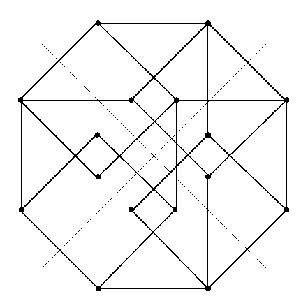
Putting the vertices of the hypercube and the hyperoctahedron together, we get all 8 + 16 = 24 elements of the binary tetrahedral group. These are the vertices of a 4-dimensional shape which is called the '24-cell' because it also has 24 octahedral faces:

But remember, the binary octahedral group is twice as big as the binary tetrahedral group! So it forms a group of 48 unit quaternions. These are the vertices of two separate 24-cells which are 'dual' to each other: the vertices of one hover above the faces of the other.
Here is an animation of the binary octahedral group, created by Greg Egan:

_tiling.png)
Mathematics is only fun for me when general theory and specific
examples go hand in hand. Theories are like lines, while examples are
like points. Each theory goes through many examples; many theories
intersect at each example.
December 27, 2021
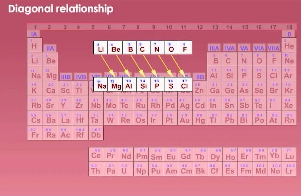
Usually each element in the periodic table is like the element below it. But sometimes it's like the element below and to the right! These are called diagonal relationships, and they're pretty weird and interesting.
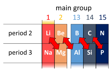
For example, boron and silicon are both semiconductors, not metals. But aluminum, directly below boron, is a conductive metal! So it's more like beryllium.
But you can get in lots of arguments here. Is carbon more like silicon or phosphorus?
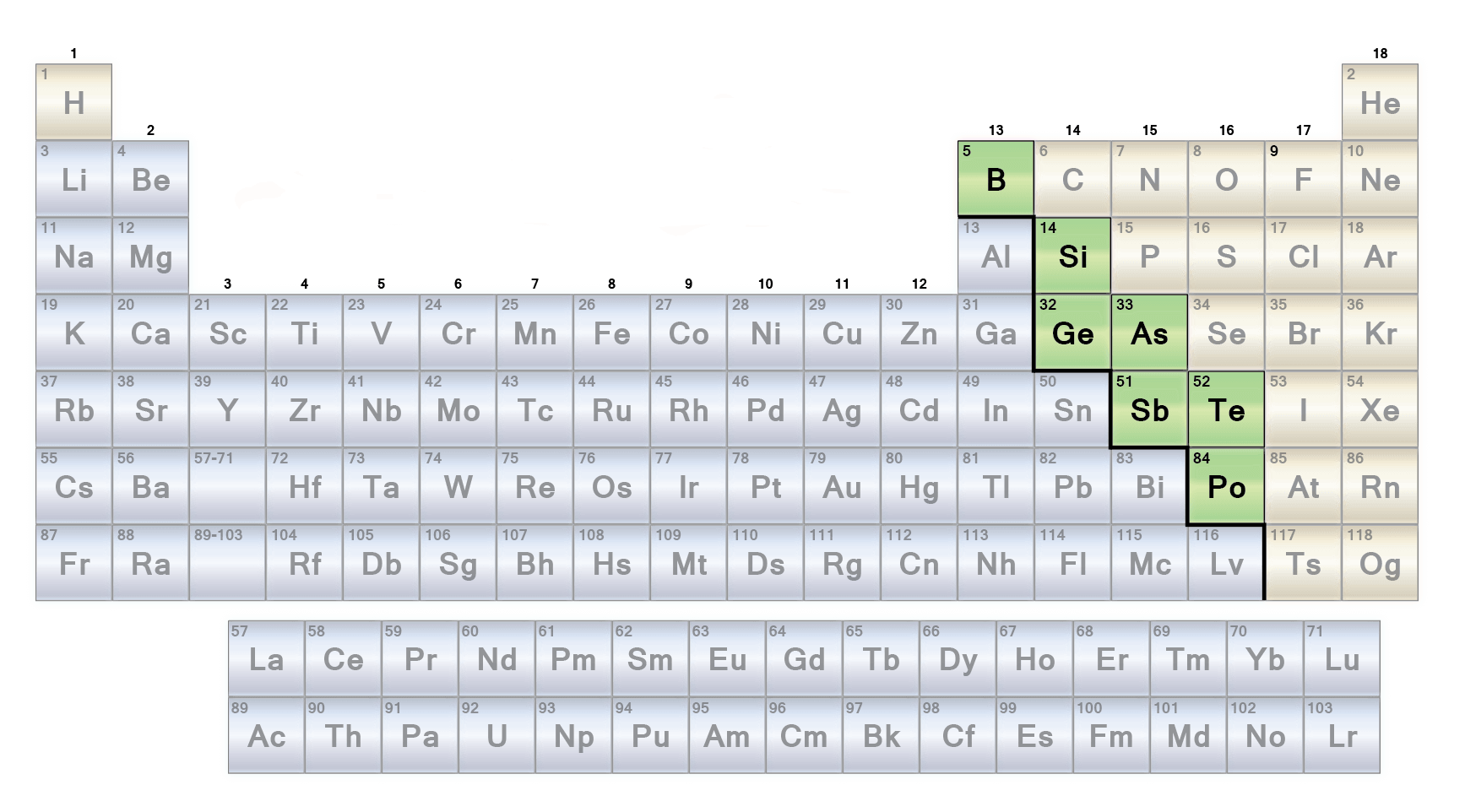
You can see this diagonal business going on with the 'semimetals', shown in green above. They're between metals and nonmetals. They're shiny like metals, but they're more brittle, and don't conduct electricity as well: they're often semiconductors!
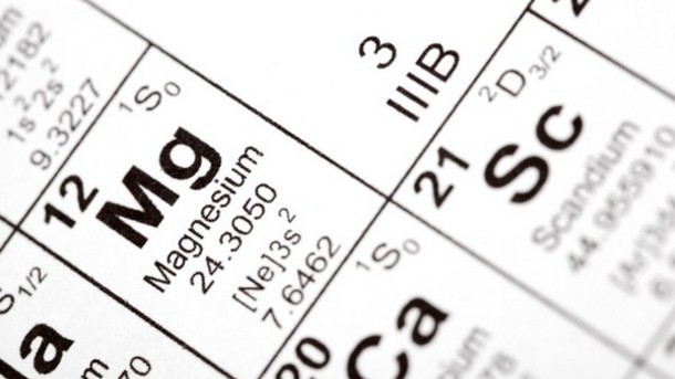
My favorite diagonal relationship is a bit less famous: scandium is a bit like magnesium! They're both shiny metals that can catch on fire and burn with a hot flame.
But what's really going on with these diagonal relationships?
When you move down the periodic table the atoms get bigger — but when you move to the right they get one more electron in their outermost subshell. So, the charge density near the edge of the atom stays roughly the same!
This creates diagonal relationships.
This idea may apply even better to ions, where you remove some electrons in the outermost subshell. For example, Li+ is a small ion with a +1 charge and Mg++ is somewhat larger with a +2 charge. So magnesium acts a lot like lithium — maybe more than sodium does!
But it's all rather complicated. If you're a mathematician you want
theorems. Chemistry is mathematical... but the math is so complicated
that we need to fall back on rules of thumb. You can find this
infuriating... or delightful.
December 28, 2021

The California rains have had a huge effect in reducing areas of extreme drought (dark red).