

|
|
|
|
Today I'll show you how a molecule can carry out a random walk on this graph. Then I'll get to work showing how any graph gives:
The trick is to use an operator called the 'graph Laplacian', a discretized version of the Laplacian which happens to be both infinitesimal stochastic and self-adjoint. As we saw in Part 12, such an operator will give rise both to a Markov process and a quantum process (that is, a one-parameter unitary group).
The most famous operator that's both infinitesimal stochastic and self-adjoint is the Laplacian, $ \nabla^2.$ Because it's both, the Laplacian shows up in two important equations: one in stochastic mechanics, the other in quantum mechanics.
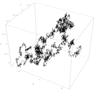
describes how the probability $ \psi(x)$ of a particle being at the point $ x$ smears out as the particle randomly walks around:
The corresponding Markov process is called 'Brownian motion'.
describes how the amplitude $ \psi(x)$ of a particle being at the point $ x$ wiggles about as the particle 'quantumly' walks around.
Both these equations have analogues where we replace space by a graph, and today I'll describe them.
Back to business! I've been telling you about the analogy between quantum mechanics and stochastic mechanics. This analogy becomes especially interesting in chemistry, which lies on the uneasy borderline between quantum and stochastic mechanics.
Fundamentally, of course, atoms and molecules are described by quantum mechanics. But sometimes chemists describe chemical reactions using stochastic mechanics instead. When can they get away with this? Apparently whenever the molecules involved are big enough and interacting with their environment enough for 'decoherence' to kick in. I won't attempt to explain this now.
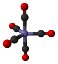
Let's imagine we have a molecule of iron pentacarbonyl with—here's the unrealistic part, but it's not really too bad—distinguishable carbonyl groups:
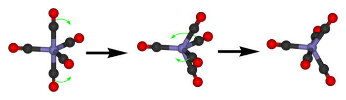
Iron pentacarbonyl is liquid at room temperatures, so as time passes, each molecule will bounce around and occasionally do a maneuver called a 'pseudorotation':
We can approximately describe this process as a random walk on a graph whose vertices are states of our molecule, and whose edges are transitions between states---namely, pseudorotations. And as we saw last time, this graph is the Desargues graph:
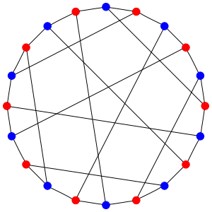
Note: all the transitions are reversible here. And thanks to the enormous amount of symmetry, the rates of all these transitions must be equal.
Let's write $ V$ for the set of vertices of the Desargues graph. A probability distribution of states of our molecule is a function
$$ \psi : V \to [0,\infty) $$with
$$ \sum_{x \in V} \psi(x) = 1 $$We can think of these probability distributions as living in this vector space:
$$ L^1(V) = \{ \psi: V \to \mathbb{R} \}$$I'm calling this space $ L^1$ because of the general abstract nonsense explained in Part 12: probability distributions on any measure space live in a vector space called $ L^1.$ Today that notation is overkill, since every function on $ V$ lies in $ L^1.$ But please humor me.
The point is that we've got a general setup that applies here. There's a Hamiltonian:
$$ H : L^1(V) \to L^1(V) $$describing the rate at which the molecule randomly hops from one state to another... and the probability distribution $ \psi \in L^1(X)$ evolves in time according to the equation:
$$ \displaystyle{ \frac{d}{d t} \psi(t) = H \psi(t) } $$But what's the Hamiltonian $ H$? It's very simple, because it's equally likely for the state to hop from any vertex to any other vertex that's connected to that one by an edge. Why? Because the problem has so much symmetry that nothing else makes sense.
So, let's write $ E$ for the set of edges of the Desargues graph. We can think of this as a subset of $ V \times V$ by saying $ (x,y) \in E$ when $ x$ is connected to $ y$ by an edge. Then
$$ \displaystyle{ (H \psi)(x) = \sum_{y \; \mathrm{such \; that} \; (x,y) \in E} \!\!\!\!\!\!\!\!\!\! \psi(y) \quad - \quad 3 \psi(x) } $$We're subtracting $ 3 \psi(x)$ because there are 3 edges coming out of each vertex $ x,$ so this is the rate at which the probability of staying at $ x$ decreases. We could multiply this Hamiltonian by a constant if we wanted the random walk to happen faster or slower... but let's not.
The next step is to solve this discretized version of the heat equation:
$$ \displaystyle{ \frac{d}{d t} \psi(t) = H \psi(t) } $$Abstractly, the solution is easy:
$$ \psi(t) = \exp(t H) \psi(0) $$But to actually compute $ \exp(t H),$ we might want to diagonalize the operator $ H.$ In this particular example, we can do this by taking advantage of the enormous symmetry of the Desargues graph. But let's not do this just yet. First let's draw some general lessons from this example.
The Hamiltonian we just saw is an example of a 'graph Laplacian'. We can write down such a Hamiltonian for any graph, but it gets a tiny bit more complicated when different vertices have different numbers of edges coming out of them.
The word 'graph' means lots of things, but right now I'm talking about simple graphs. Such a graph has a set of vertices $ V$ and a set of edges $ E \subseteq V \times V,$ such that
$$ (x,y) \in E \Rightarrow (y,x) \in E $$which says the edges are undirected, and
$$ (x,x) \notin E $$which says there are no loops. Let $ d(x)$ be the degree of the vertex $ x,$ meaning the number of edges coming out of it.
Then the graph Laplacian is this operator on $ L^1(V)$:
$$ \displaystyle{ (H \psi)(x) = \sum_{y \; \mathrm{such \; that} \; (x,y) \in E} \!\!\!\!\!\!\!\!\!\! \psi(y) \quad - \quad d(x) \psi(x) } $$There is a huge amount to say about graph Laplacians! If you want, you can get started here:
But for now, let's just say that $ \exp(t H)$ is a Markov process describing a random walk on the graph, where hopping from one vertex to any neighboring vertex has unit probability per unit time. We can make the hopping faster or slower by multiplying $ H$ by a constant. And here is a good time to admit that most people use a graph Laplacian that's the negative of ours, and write time evolution as $ \exp(-t H)$. The advantage is that then the eigenvalues of the Laplacian are $ \ge 0.$
But what matters most is this. We can write the operator $ H$ as a matrix whose entry $ H_{x y}$ is 1 when there's an edge from $ x$ to $ y$ and 0 otherwise, except when $ x = y$, in which case the entry is $ -d(x).$ And then:
Puzzle 1. Show that for any finite graph, the graph Laplacian $ H$ is infinitesimal stochastic, meaning that:
$$ \displaystyle{ \sum_{x \in V} H_{x y} = 0 } $$and
$$ x \ne y \Rightarrow H_{x y} \ge 0 $$This fact implies that for any $ t \ge 0,$ the operator $ \exp(t H)$ is stochastic—just what we need for a Markov process.
But we could also use $ H$ as a Hamiltonian for a quantum system, if we wanted. Now we think of $ \psi(x)$ as the amplitude for being in the state $ x \in V$. But now $ \psi$ is a function
$$ \psi : V \to \mathbb{C} $$with
$$ \displaystyle{ \sum_{x \in V} |\psi(x)|^2 = 1 } $$We can think of this function as living in the Hilbert space
$$ L^2(V) = \{ \psi: V \to \mathbb{C} \} $$where the inner product is
$$ \langle \phi, \psi \rangle = \sum_{x \in V} \overline{\phi(x)} \psi(x) $$Puzzle 2. Show that for any finite graph, the graph Laplacian $ H: L^2(V) \to L^2(V)$ is self-adjoint, meaning that:
$$ H_{x y} = \overline{H}_{y x} $$This implies that for any $ t \in \mathbb{R}$, the operator $ \exp(-i t H)$ is unitary—just what we need for one-parameter unitary group. So, we can take this version of Schrödinger's equation:
$$ \displaystyle{ \frac{d}{d t} \psi = -i H \psi } $$and solve it:
$$ \displaystyle{ \psi(t) = \exp(-i t H) \psi(0) } $$and we'll know that time evolution is unitary!
So, we're in a dream world where we can do stochastic mechanics and quantum mechanics with the same Hamiltonian. I'd like to exploit this somehow, but I'm not quite sure how. Of course physicists like to use a trick called Wick rotation where they turn quantum mechanics into stochastic mechanics by replacing time by imaginary time. We can do that here. But I'd like to do something new, special to this context.
Maybe I should learn more about chemistry and graph theory. Of course, graphs show up in at least two ways: first for drawing molecules, and second for drawing states and transitions, as I've been doing. These books are supposed to be good:
The second is apparently the magisterial tome of the subject. The prices of these books are absurd: for example, Amazon sells the first for 300 dollars, and the second for 222. Luckily the university here should have them...
Greg Egan figured out a nice way to explicitly describe the eigenvectors of the Laplacian $H$ for the Desargues graph. This lets us explicitly solve the heat equation
$$ \displaystyle{ \frac{d}{d t} \psi = H \psi } $$and also the Schrödinger equation on this graph.
First there is an obvious eigenvector: any constant function. Indeed, for any finite graph, any constant function $\psi$ is an eigenvector of the graph Laplacian with eigenvalue zero:
$$H \psi = 0$$so that
$$ \exp(t H) \psi = \psi $$This reflects the fact that the evenly smeared probability distribution is an equilibrium state for the random walk described by heat equation. For a connected graph this will be the only equilibrium state. For a graph with several connected components, there will be an equilibrum state for each connected component, which equals some positive constant on that component and zero elsewhere.
For the Desargues graph, or indeed any connected graph, all the other eigenvectors will be functions that undergo exponential decay at various rates: $$H \psi = \lambda \psi $$ with $\lambda \lt 0$, so that $$\exp(t H) \psi = \exp(\lambda t) \psi $$
decays as $t$ increases. But since probability is conserved, any vector that undergoes exponential decay must have terms that sum to zero. So a vector like this won't be a stochastic state, but rather a deviation from equilibrium. We can write any stochastic state as the equilibrium state plus a sum of terms that decay with different rate constants.
If you put a value of 1 on every red dot and -1 on every blue dot, you get an eigenvector of the Hamiltonian with eigenvalue -6: -3 for the diagonal entry for each vertex, and -3 for the sum over the neighbors.
By trial and error, it's not too hard to find examples of variations on this where some vertices have a value of zero. Every vertex with zero either has its neighbors all zero, or two neighbors of opposite signs:
So the general pattern is what you'd expect: the more neighbors of equal value each non-zero vertex has, the more slowly that term will decay.
In more detail, the eigenvectors are given by the the following functions, together with functions obtained by rotating these pictures. Unlabelled dots are labelled by zero:
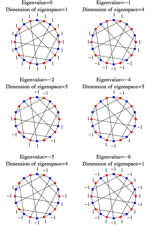
In fact you can span the eigenspaces by rotating the particular eigenvectors I drew by successive multiples of 1/5 of a rotation, i.e. 4 dots.
If you do this for the examples with eigenvalues -2 and -4, it's not too hard to see that all five rotated diagrams are linearly independent. If you do it for the examples with eigenvalues -1 and -5, four rotated diagrams are linearly independent. So along with the two 1-dimensional spaces, that's enough to prove that you've exhausted the whole 20-dimensional space.
You can also read comments on Azimuth, and make your own comments or ask questions there!
|
|
|
|