

|
|
|
|
Our example won't show how powerful this theorem is: it's too simple. But it'll help explain the ideas involved.
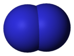
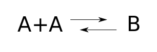
A diatomic molecule consists of two atoms of the same kind, stuck together:
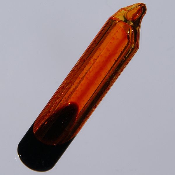
At room temperature there are 5 elements that are diatomic gases: hydrogen, nitrogen, oxygen, fluorine, chlorine. Bromine is a diatomic liquid, but easily evaporates into a diatomic gas:
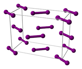
Iodine is a crystal at room temperatures:
but if you heat it a bit, it becomes a diatomic liquid and then a gas:
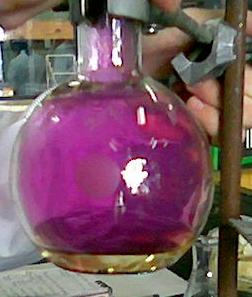
so people often list it as a seventh member of the diatomic club.
When you heat any diatomic gas enough, it starts becoming a 'monatomic' gas as molecules break down into individual atoms. However, just as a diatomic molecule can break apart into two atoms: $$ A_2 \to A + A $$ two atoms can recombine to form a diatomic molecule: $$ A + A \to A_2 $$ So in equilibrium, the gas will be a mixture of diatomic and monatomic forms. The exact amount of each will depend on the temperature and pressure, since these affect the likelihood that two colliding atoms stick together, or a diatomic molecule splits apart. The detailed nature of our gas also matters, of course.
But we don't need to get into these details here! Instead, we can just write down the 'rate equation' for the reactions we're talking about. All the details we're ignoring will be hiding in some constants called 'rate constants'. We won't try to compute these; we'll leave that to our chemist friends.
To write down our rate equation, we start by drawing a 'reaction network'. For this, we can be a bit abstract and call the diatomic molecule $B$ instead of $A_2$. Then it looks like this:
We could write down the same information using a Petri net:
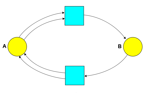
But today let's focus on the reaction network! Staring at this picture, we can read off various things:
• Species. The species are the different kinds of atoms, molecules, etc. In our example the set of species is $S = \{A, B\}$.
• Complexes. A complex is finite sum of species, like $A$, or $A + A$, or for a fancier example using more efficient notation, $2 A + 3 B$. So, we can think of a complex as a vector $v \in \mathbb{R}^S$. The complexes that actually show up in our reaction network form a set $C \subseteq \mathbb{R}^S$. In our example, $C = \{A+A, B\}$.
• Reactions. A reaction is an arrow going from one complex to another. In our example we have two reactions: $A + A \to B$ and $B \to A + A$. Chemists define a reaction network to be a triple $(S, C, T)$ where $S$ is a set of species, $C$ is the set of complexes that appear in the reactions, and $T$ is the set of reactions $v \to w$ where $v, w \in C$. (Stochastic Petri net people call reactions transitions, hence the letter $T$.)
So, in our example we have:
• Species $S = \{A,B\}$.
• Complexes: $C= \{A+A, B\}$.
• Reactions: $T = \{A+A\to B, B\to A+A\}$. To get the rate equation, we also need one more piece of information: a rate constant $r(\tau)$ for each reaction $\tau \in T$. This is a nonnegative real number that affects how fast the reaction goes. All the details of how our particular diatomic gas behaves at a given temperature and pressure are packed into these constants!
The rate equation says how the expected numbers of the various species—atoms, molecules and the like—changes with time. This equation is deterministic. It's a good approximation when the numbers are large and any fluctuations in these numbers are negligible by comparison.
Here's the general form of the rate equation:
$$ \frac{d}{d t} x_i = \sum_{\tau\in T} r(\tau) \, (n_i(\tau)-m_i(\tau)) \, x^{m(\tau)} $$
Let's take a closer look. The quantity $x_i$ is the expected population of the $i$th species. So, this equation tells us how that changes. But what about the right hand side? As you might expect, it's a sum over reactions. And:
• The term for the reaction $\tau$ is proportional to the rate constant $r(\tau)$.
• Each reaction $\tau$ goes between two complexes, so we can write it as $m(\tau) \to n(\tau)$. Among chemists the input $m(\tau)$ is called the reactant complex, and the output is called the product complex. The difference $n_i(\tau)-m_i(\tau)$ tells us how many items of species $i$ get created, minus how many get destroyed. So, it's the net amount of this species that gets produced by the reaction $\tau$. The term for the reaction $\tau$ is proportional to this, too.
• Finally, the law of mass action says that the rate of a reaction is proportional to the product of the concentrations of the species that enter as inputs. More precisely, if we have a reaction $\tau$ with input is the complex $m(\tau)$, we define $ x^{m(\tau)} = x_1^{m_1(\tau)} \cdots x_k^{m_k(\tau)}$. The law of mass action says the term for the reaction $\tau$ is proportional to this, too!
Let's see what this says for the reaction network we're studying:
Let's write $x_1(t)$ for the number of $A$ atoms and $x_2(t)$ for the number of $B$ molecules. Let the rate constant for the reaction $B \to A + A$ be $\alpha$, and let the rate constant for $A + A \to B$ be $\beta$. Then the rate equation is this:
$$ \frac{d}{d t} x_1 = 2 \alpha x_2 - 2 \beta x_1^2 $$
$$ \frac{d}{d t} x_2 = -\alpha x_2 + \beta x_1^2 $$
This is a bit intimidating. However, we can solve it in closed form thanks to something very precious: a conserved quantity.
We've got two species, $A$ and $B$. But remember, $B$ is just an abbreviation for a molecule made of two $A$ atoms. So, the total number of $A$ atoms is conserved by the reactions in our network. This is the number of $A$'s plus twice the number of $B$'s: $x_1 + 2x_2$. So, this should be a conserved quantity: it should not change with time. Indeed, by adding the first equation above to twice the second, we see:
$$ \frac{d}{d t} \left( x_1 + 2x_2 \right) = 0 $$
As a consequence, any solution will stay on a line
$$ x_1 + 2 x_2 = c $$
for some constant $c$. We can use this fact to rewrite the rate equation just in terms of $x_1$:
$$ \frac{d}{d t} x_1 = \alpha (2c - x_1) - 2 \beta x_1^2 $$
This is a separable differential equation, so we can solve it if we can figure out how to do this integral
$$ t = \int \frac{d x_1}{\alpha (2c - x_1) - 2 \beta x_1^2 } $$
and then solve for $x_1$.
This sort of trick won't work for more complicated examples. But the idea remains important: the numbers of atoms of various kinds—hydrogen, helium, lithium, and so on—are conserved by chemical reactions, so a solution of the rate equation can't roam freely in $\mathbb{R}^S$. It will be trapped on some hypersurface, which is called a 'stoichiometric compatibility class'. And this is very important.
We don't feel like doing the integral required to solve our rate equation in closed form, because this idea doesn't generalize too much. On the other hand, we can always solve the rate equation numerically. So let's try that!
For example, suppose we set $\alpha = \beta = 1$. We can plot the solutions for three different choices of initial conditions, say $(x_1,x_2) = (0,3), (4,0),$ and $(3,3)$. We get these graphs:
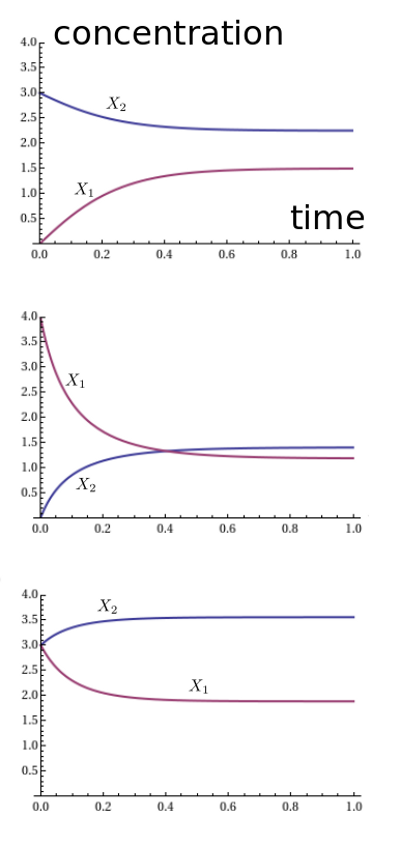
It looks like the solution always approaches an equilibrium. We seem to be getting different equilibria for different initial conditions, and the pattern is a bit mysterious. However, something nice happens when we plot the ratio $x_1^2 / x_2$:
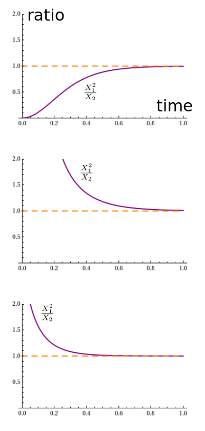
Apparently it always converges to 1. Why should that be? It's not terribly surprising. With both rate constants equal to 1, the reaction $A + A \to B$ proceeds at a rate equal to the square of the number of $A$'s, namely $x_1^2$. The reverse reaction proceeds at a rate equal to the number of $B$'s, namely $x_2$. So in equilibrium, we should have $x_1^2 = x_2$.
But why is the equilibrium stable? In this example we could see that using the closed-form solution, or maybe just common sense. But it also follows from a powerful theorem that handles a lot of reaction networks.
It's called Feinberg's deficiency zero theorem, and we saw it last time. Very roughly, it says that if our reaction network is 'weakly reversible' and has 'deficiency zero', the rate equation will have equilibrium solutions that behave about as nicely as you could want.
Let's see how this works. We need to remember some jargon:
• Weakly reversible. A reaction network is weakly reversible if for every reaction $v \to w$ in the network, there exists a path of reactions in the network starting at $w$ and leading back to $v$.
• Reversible. A reaction network is reversible if for every reaction $v \to w$ in the network, $w \to v$ is also a reaction in the network. Any reversible reaction network is weakly reversible. Our example is reversible, since it consists of reactions $A + A \to B$, $B \to A + A$.
But what about 'deficiency zero'? We defined that concept last time, but let's review:
• Connected component. A reaction network gives a kind of graph with complexes as vertices and reactions as edges. Two complexes lie in the same connected component if we can get from one to the other by a path of reactions, where at each step we're allowed to go either forward or backward along a reaction. Chemists call a connected component a linkage class. In our example there's just one:
• Stoichiometric subspace. The stoichiometric subspace is the subspace $\mathrm{Stoch} \subseteq \mathbb{R}^S$ spanned by the vectors of the form $w - v$ for all reactions $v \to w$ in our reaction network. This subspace describes the directions in which a solution of the rate equation can move. In our example, it's spanned by $B - 2 A$ and $2 A - B$, or if you prefer, $(-2,1)$ and $(2,-1)$. These vectors are linearly dependent, so the stoichiometric subspace has dimension 1.
• Deficiency. The deficiency of a reaction network is the number of complexes, minus the number of connected components, minus the dimension of the stoichiometric subspace. In our example there are 2 complexes, 1 connected component, and the dimension of the stoichiometric subspace is 1. So, our reaction network has deficiency 2 - 1 - 1 = 0.
So, the deficiency zero theorem applies! What does it say? To understand it, we need a bit more jargon. First of all, a vector $x \in \mathbb{R}^S$ tells us how much we've got of each species: the amount of species $i \in S$ is the number $x_i$. And then:
• Stoichiometric compatibility class. Given a vector $v\in \mathbb{R}^S$, its stoichiometric compatibility class is the subset of all vectors that we could reach using the reactions in our reaction network:
$$ \{ v + w \; : \; w \in \mathrm{Stoch} \} $$
In our example, where the stoichiometric subspace is spanned by $(2,-1)$, the stoichiometric compatibility class of the vector $(a,b)$ is the line consisting of points
$$ (x_1, x_2) = (a,b) + s(2,-1) $$
where the parameter $s$ ranges over all real numbers. Notice that this line can also be written as
$$ x_1 + 2x_2 = c $$
We've already seen that if we start with initial conditions on such a line, the solution will stay on this line. And that's how it always works: as time passes, any solution of the rate equation stays in the same stoichiometric compatibility class!
In other words: the stoichiometric subspace is defined by a bunch of linear equations, one for each linear conservation law that all the reactions in our network obey.
Here a linear conservation law is a law saying that some linear combination of the numbers of species does not change.
Next:
• Positivity. A vector in $\mathbb{R}^S$ is positive if all its components are positive; this describes a a container of chemicals where all the species are actually present. The positive stoichiometric compatibility class of $x\in \mathbb{R}^S$ consists of all positive vectors in its stoichiometric compatibility class.
We finally have enough jargon in our arsenal to state the zero deficiency theorem. We'll only state the part we need today:
Zero Deficiency Theorem (Feinberg). If a reaction network is weakly reversible and the rate constants are positive, the rate equation has exactly one equilibrium solution in each positive stoichiometric compatibility class. Any sufficiently nearby solution that starts in the same class will approach this equilibrium as $t \to +\infty$.
In our example, this theorem says there's just one positive equilibrium $(x_1,x_2)$ in each line
$$ x_1 + 2x_2 = c $$
We can find it by setting the time derivatives to zero:
$$ \frac{d}{d t} x_1 = 2 \alpha x_2 - 2 \beta x_1^2 = 0 $$
$$ \frac{d}{d t} x_2 = -\alpha x_2 + \beta x_1^2 = 0 $$
Solving these, we get
$$ \frac{x_1^2}{x_2} = \frac{\alpha}{\beta} $$
So, these are our equilibrium solutions. It's easy to verify that indeed, there's one of these in each stoichiometric compatibility class $x_1 + 2x_2 = c$. And the zero deficiency theorem also tells us that any sufficiently nearby solution that starts in the same class will approach this equilibrium as $t \to \infty$.
This partially explains what we saw before in our graphs. It shows that in the case $\alpha = \beta = 1$, any solution that starts by nearly having
$$ \frac{x_1^2}{x_2} = 1 $$
will actually have
$$ \lim_{t \to +\infty} \frac{x_1^2}{x_2} = 1 $$
But in fact, in this example we don't even need to start near the equilibrium for our solution to approach the equilibrium! What about in general? We don't know, but just to get the ball rolling, we'll risk the following wild guess:
Conjecture. If a reaction network is weakly reversible and the rate constants are positive, the rate equation has exactly one equilibrium solution in each positive stoichiometric compatibility class, and any positive solution that starts in the same class will approach this equilibrium as $t \to +\infty$.
If anyone knows a proof or counterexample, we'd be interested. If this result were true, it would really clarify the dynamics of reaction networks in the zero deficiency case.
Next time we'll talk about this same reaction network from a stochastic point of view, where we think of the atoms and molecules as reacting in a probabilistic way. And we'll see how the conservation laws we've been talking about today are related to Noether's theorem for Markov processes!
You can also read comments on Azimuth, and make your own comments or ask questions there!
|
|
|
|