July 18, 2012

Network Theory (Part 19)

John Baez and Jacob Biamonte

Last time we started looking at a simple example: a diatomic gas.

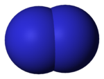
A diatomic molecule of this gas can break apart into two atoms:

$$ A_2 \to A + A $$

and conversely, two atoms can combine to form a diatomic molecule:

$$ A + A \to A_2 $$

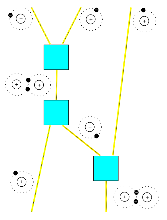
We can draw both these reactions using a chemical reaction network:

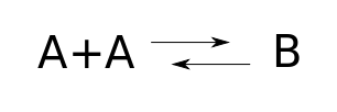
where we're writing $B$ instead of $A_2$ to abstract away some detail that's just distracting here.

Last time we looked at the rate equation for this chemical reaction network, and found equilibrium solutions of that equation. Now let's look at the master equation, and find equilibrium solutions of that. This will serve as a review of three big theorems.

The master equation

We'll start from scratch. The master equation is all about how atoms or molecules or rabbits or wolves or other things interact randomly and turn into other things. So, let's write $\psi_{m,n}$ for the probability that we have $m$ atoms of $A$ and $n$ molecule of $B$ in our container. These probabilities are functions of time, and master equation will say how they change.

First we need to pick a rate constant for each reaction. Let's say the rate constant for the reaction that produces $A$s is some number $\alpha > 0$:

$$ B \to A + A $$

while the rate constant for the reaction that produces $B$s is some number $\beta > 0$:

$$ A + A \to B $$

Before we make it pretty using the ideas we've been explaining all along, the master equation says:

Yuck!

Normally we don't show you such nasty equations. Indeed the whole point of our work has been to demonstrate that by packaging the equations in a better way, we can understand them using high-level concepts instead of mucking around with millions of scribbled symbols. But we thought we'd show you what's secretly lying behind our beautiful abstract formalism, just once.

Each term has a meaning. For example, the third one:

$$ \beta (m+2)(m+1)\psi_{m+2,n-1}(t) $$

means that the reaction $A + A \to B$ will tend to increase the probability of there being $m$ atoms of $A$ and $n$ molecules of $B$ if we start with $m+2$ atoms of $A$ and $n-1$ molecules of $B.$ This reaction can happen in $(m+2)(m+1)$ ways. And it happens at a probabilistic rate proportional to the rate constant for this reaction, $\beta$.

We won't go through the rest of the terms. It's a good exercise to do so, but there could easily be a typo in the formula, since it's so long and messy. So let us know if you find one!

To simplify this mess, the key trick is to introduce a generating function that summarizes all the probabilities in a single power series:

$$ \Psi = \sum_{m,n \ge 0} \psi_{m,n} y^m \, z^n $$

It's a power series in two variables, $y$ and $z,$ since we have two chemical species: $A$s and $B$s.

Using this trick, the master equation looks like

$$ \displaystyle{ \frac{d}{d t} \Psi(t) = H \Psi(t) } $$

where the Hamiltonian $H$ is a sum of terms, one for each reaction. This Hamiltonian is built from operators that annihilate and create $A$s and $B$s. The annihilation and creation operators for $A$ atoms are:

$$ \displaystyle{ a = \frac{\partial}{\partial y} , \qquad a^\dagger = y } $$

The annihilation operator differentiates our power series with respect to the variable $y.$ The creation operator multiplies it by that variable. Similarly, the annihilation and creation operators for $B$ molecules are:

$$ \displaystyle{ b = \frac{\partial}{\partial z} , \qquad b^\dagger = z } $$

In Part 8 we explained a recipe that lets us stare at our chemical reaction network and write down this Hamiltonian:

$$ H = \alpha ({a^\dagger}^2 b - b^\dagger b) + \beta (b^\dagger a^2 - {a^\dagger}^2 a^2) $$

As promised, there's one term for each reaction. But each term is itself a sum of two: one that increases the probability that our container of chemicals will be in a new state, and another that decreases the probability that it's in its original state. We get a total of four terms, which correspond to the four terms in our previous way of writing the master equation.

Puzzle 1. Show that this new way of writing the master equation is equivalent to the previous one.

Equilibrium solutions

Now we will look for all equilibrium solutions of the master equation: in other words, solutions that don't change with time. So, we're trying to solve

$$ H \Psi = 0 $$

Given the rather complicated form of the Hamiltonian, this seems tough. The challenge looks more concrete but even more scary if we go back to our original formulation. We're looking for probabilities $\psi_{m,n},$ nonnegative numbers that sum to one, such that $$ \alpha (n+1) \, \psi_{m-2,n+1} \; - \; \alpha n \, \psi_{m,n} \; + \; \beta (m+2)(m+1) \, \psi_{m+2,n-1} \; - \;\beta m(m-1) \, \psi_{m,n} = 0 $$

This equation is horrid! But the good news is that it's linear, so a linear combination of solutions is again a solution. This lets us simplify the problem using a conserved quantity.

Clearly, there's a quantity that the reactions here don't change:

What's that? It's the number of $A$s plus twice the number of $B$s. After all, a $B$ can turn into two $A$s, or vice versa.

(Of course the secret reason is that $B$ is a diatomic molecule made of two $A$s. But you'd be able to follow the logic here even if you didn't know that, just by looking at the chemical reaction network... and sometimes this more abstract approach is handy! Indeed, the way chemists first discovered that certain molecules are made of certain atoms is by seeing which reactions were possible and which weren't.)

Suppose we start in a situation where we know for sure that the number of $B$s plus twice the number of $A$s equals some number $k$:

$$ \psi_{m,n} = 0 \; \textrm{unless} \; m+2n = k $$

Then we know $\Psi$ is initially of the form

$$ \Psi = \sum_{m+2n = k} \psi_{m,n} \, y^m z^n $$

But since the number of $A$s plus twice the number of $B$s is conserved, if $\Psi$ obeys the master equation it will continue to be of this form!

Put a fancier way, we know that if a solution of the master equation starts in this subspace:

$$ L_k = \{ \Psi: \; \Psi = \sum_{m+2n = k} \psi_{m,n} y^m z^n \; \textrm{for some} \; \psi_{m,n} \} $$

it will stay in this subspace. So, because the master equation is linear, we can take any solution $\Psi$ and write it as a linear combination of solutions $\Psi_k,$ one in each subspace $L_k.$

In particular, we can do this for an equilibrium solution $\Psi.$ And then all the solutions $\Psi_k$ are also equilibrium solutions: they're linearly independent, so if one of them changed with time, $\Psi$ would too.

This means we can just look for equilibrium solutions in the subspaces $L_k.$ If we find these, we can get all equilibrium solutions by taking linear combinations.

Once we've noticed that, our horrid equation makes a bit more sense:

$$ \alpha (n+1) \, \psi_{m-2,n+1} \; - \; \alpha n \, \psi_{m,n} \; + \; \beta (m+2)(m+1) \, \psi_{m+2,n-1} \; - \;\beta m(m-1) \, \psi_{m,n} = 0 $$

Note that if the pair of subscripts $m, n$ obey $m + 2n = k,$ the same is true for the other pairs of subscripts here! So our equation relates the values of $\psi_{m,n}$ for all the points $(m,n)$ with integer coordinates lying on this line segment:

You should be visualizing something like this:

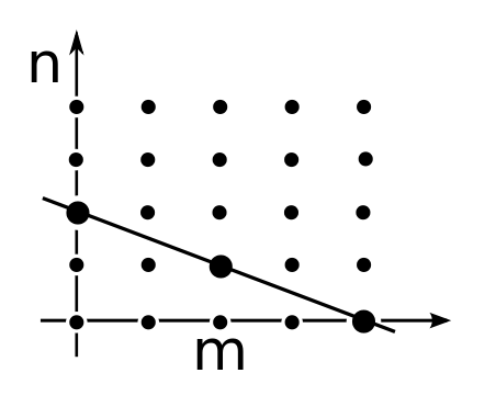
If you think about it a minute, you'll see that if we know $\psi_{m,n}$ at two points on such a line, we can keep using our equation to recursively work out all the rest. So, there are at most two linearly independent equilibrium solutions of the master equation in each subspace $L_k.$

Why at most two? Why not two? Well, we have to be a bit careful about what happens at the ends of the line segment: remember that $\psi_{m,n}$ is defined to be zero when $m$ or $n$ becomes negative. If we think very hard about this, we'll see there's just one linearly independent equilibrium solution of the master equation in each subspace $L_k.$ But this is the sort of nitty-gritty calculation that's not fun to watch someone else do, so we won't bore you with that.

Soon we'll move on to a more high-level approach to this problem. But first, one remark. Our horrid equation is like a fancy version of the usual discretized form of the equation

$$ \displaystyle {\frac{d^2 \psi}{d x^2} = 0 } $$

namely:

$$ \psi_{n-1} - 2 \psi_{n} + \psi_{n+1} = 0 $$

And this makes sense, since we get

$$ \displaystyle {\frac{d^2 \psi}{d x^2} = 0 } $$

by taking the heat equation:

$$ \displaystyle \frac{\partial \psi}{\partial t} = {\frac{\partial^2 \psi}{\partial x^2} } $$

and assuming $\psi$ doesn't depend on time. So what we're doing is a lot like looking for equilibrium solutions of the heat equation.

The heat equation describes how heat smears out as little particles of heat randomly move around. True, there don't really exist 'little particles of heat', but this equation also describes the diffusion of any other kind of particles as they randomly move around undergoing Brownian motion. Similarly, our master equation describes a random walk on this line segment:

$$ m+2n = k , \qquad m , n \ge 0 $$

or more precisely, the points on this segment with integer coordinates. The equilibrium solutions arise when the probabilities $\psi_{m,n}$ have diffused as much as possible.

If you think about it this way, it should be physically obvious that there's just one linearly independent equilibrium solution of the master equation for each value of $k.$

There's a general moral here, too, which we're seeing in a special case: the master equation for a chemical reaction network really describes a bunch of random walks, one for each allowed value of the conserved quantities that can be built as linear combinations of number operators. In our case we have one such conserved quantity, but in general there may be more (or none).

Furthermore, these 'random walks' are what we've been calling Markov processes.

Noether's theorem

We simplified our task of finding equilibrium solutions of the master equation by finding a conserved quantity. The idea of simplifying problems using conserved quantities is fundamental to physics: this is why physicists are so enamored with quantities like energy, momentum, angular momentum and so on.

Nowadays physicists often use 'Noether's theorem' to get conserved quantities from symmetries. There's a very simple version of Noether's theorem for quantum mechanics, but in Part 11 we saw a version for stochastic mechanics, and it's that version that is relevant now. Here's a paper which explains it in detail:

• John Baez and Brendan Fong, Noether's theorem for Markov processes.

We don't really need Noether's theorem now, since we found the conserved quantity and exploited it without even noticing the symmetry. Nonetheless it's interesting to see how it relates to what we're doing.

For the reaction we're looking at now, the idea is that the subspaces $L_k$ are eigenspaces of an operator that commutes with the Hamiltonian $H.$ It follows from standard math that a solution of the master equation that starts in one of these subspaces, stays in that subspace.

What is this operator? It's built from 'number operators'. The number operator for $A$s is

$$ N_A = a^\dagger a $$

and the number operator for $B$s is

$$ N_B = b^\dagger b $$

A little calculation shows

$$ N_A \,y^m z^n = m \, y^m z^n, \quad \qquad N_B\, y^m z^n = n \,y^m z^n $$

so the eigenvalue of $N_A$ is the number of $A$s, while the eigenvalue of $N_B$ is the number of $B$s. This is why they're called number operators.

As a consequence, the eigenvalue of the operator $N_A + 2N_B$ is the number of $A$s plus twice the number of $B$s:

$$ (N_A + 2N_B) \, y^m z^n = (m + 2n) \, y^m z^n $$

Let's call this operator $O,$ since it's so important:

$$ O = N_A + 2N_B $$

If you think about it, the spaces $L_k$ we saw a minute ago are precisely the eigenspaces of this operator:

$$ L_k = \{ \Psi : \; O \Psi = k \Psi \} $$

As we've seen, solutions of the master equation that start in one of these eigenspaces will stay there. This lets take some techniques that are very familiar in quantum mechanics, and apply them to this stochastic situation.

First of all, time evolution as described by the master equation is given by the operators $\exp(t H).$ In other words,

$$ \displaystyle{ \frac{d}{d t} \Psi(t) } = H \Psi(t) \quad \textrm{and} \quad \Psi(0) = \Phi \quad \Rightarrow \quad \Psi(t) = \exp(t H) \Phi $$

But if you start in some eigenspace of $O,$ you stay there. Thus if $\Phi$ is an eigenvector of $O,$ so is $\exp(t H) \Phi,$ with the same eigenvalue. In other words,

$$ O \Phi = k \Phi $$

implies

$$ O \exp(t H) \Phi = k \exp(t H) \Phi = \exp(t H) O \Phi $$

But since we can choose a basis consisting of eigenvectors of $O,$ we must have

$$ O \exp(t H) = \exp(t H) O $$

or, throwing caution to the winds and differentiating:

$$ O H = H O $$

So, as we'd expect from Noether's theorem, our conserved quantity commutes with the Hamiltonian! This in turn implies that $H$ commutes with any polynomial in $O,$ which in turn suggests that

$$ \exp(s O) H = H \exp(s O) $$

and also

$$ \exp(s O) \exp(t H) = \exp(t H) \exp(s O) $$

The last equation says that $O$ generates a 1-parameter family of 'symmetries': operators $\exp(s O)$ that commute with time evolution. But what do these symmetries actually do? Since

$$ O y^m z^n = (m + 2n) y^m z^n $$

we have

$$ \exp(s O) y^m z^n = e^{s(m + 2n)}\, y^m z^n $$

So, this symmetry takes any probability distribution $\psi_{m,n}$ and multiplies it by $e^{s(m + 2n)}.$

In other words, our symmetry multiplies the relative probability of finding our container of gas in a given state by a factor of $e^s$ for each $A$ atom, and by a factor of $e^{2s}$ for each $B$ molecule. It might not seem obvious that this operation commutes with time evolution! However, experts on chemical reaction theory are familiar with this fact.

Finally, a couple of technical points. Starting where we said "throwing caution to the winds", our treatment has not been rigorous, since $O$ and $H$ are unbounded operators, and these must be handled with caution. Nonetheless, all the commutation relations we wrote down are true.

The operators $\exp(s O)$ are unbounded for positive $s.$ They're bounded for negative $s,$ so they give a one-parameter semigroup of bounded operators. But they're not stochastic operators: even for $s$ negative, they don't map probability distributions to probability distributions. However, they do map any nonzero vector $\Psi$ with $\psi_{m,n} \ge 0$ to a vector $\exp(s O) \Psi$ with the same properties. So, we can just normalize this vector and get a probability distribution. The need for this normalization is why we spoke of relative probabilities.

The Anderson–Craciun–Kurtz theorem

Now we'll actually find all equilibrium solutions of the master equation in closed form. To understand this final section, you really do need to remember some things we've discussed earlier. Last time we considered the same chemical reaction network we're studying today, but we looked at its rate equation, which looks like this:

$$ \displaystyle{ \frac{d}{d t} x_1 = 2 \alpha x_2 - 2 \beta x_1^2} $$

$$ \displaystyle{ \frac{d}{d t} x_2 = - \alpha x_2 + \beta x_1^2 } $$

This describes how the number of $A$s and $B$s changes in the limit where there are lots of them and we can treat them as varying continuously, in a deterministic way. The number of $A$s is $x_1,$ and the number of $B$s is $x_2.$

We saw that the quantity

$$ x_1 + 2 x_2 $$

is conserved, just as today we've seen that $N_A + 2 N_B$ is conserved. We saw that the rate equation has one equilibrium solution for each choice of $x_1 + 2 x_2.$ And we saw that these equilibrium solutions obey

$$ \displaystyle{ \frac{x_1^2}{x_2} = \frac{\alpha}{\beta} } $$

The Anderson–Craciun–Kurtz theorem, introduced in Part 9, is a powerful result that gets equilibrium solution of the master equation from equilibrium solutions of the rate equation. It only applies to equilibrium solutions that are 'complex balanced', but that's okay:

Puzzle 2. Show that the equilibrium solutions of the rate equation for the chemical reaction network

are complex balanced.

So, given any equilibrium solution $(x_1,x_2)$ of our rate equation, we can hit it with the Anderson-Craciun-Kurtz theorem and get an equilibrium solution of the master equation! And it looks like this:

$$ \displaystyle{ \Psi = e^{-(x_1 + x_2)} \, \sum_{m,n \ge 0} \frac{x_1^m x_2^n} {m! n! } \, y^m z^n } $$

In this solution, the probability distribution

$$ \displaystyle{ \psi_{m,n} = e^{-(x_1 + x_2)} \, \frac{x_1^m x_2^n} {m! n! } } $$

is a product of Poisson distributions. The factor in front is there to make the numbers $\psi_{m,n}$ add up to one. And remember, $x_1, x_2$ are any nonnegative numbers with

$$ \displaystyle{ \frac{x_1^2}{x_2} = \frac{\alpha}{\beta} } $$

So from all we've said, the above formula gives an explicit closed-form solution of the horrid equation

$$ \alpha (m+2)(m+1) \, \psi_{m+2,n-1} \; - \;\alpha m(m-1) \, \psi_{m,n} \; + \; \beta (n+1) \, \psi_{m-2,n+1} \; - \; \beta n \, \psi_{m,n} = 0 $$

That's pretty nice. We found some solutions without ever doing any nasty calculations.

But we've really done better than getting some equilibrium solutions of the master equation. By restricting attention to $n,m$ with $m+2n = k,$ our formula for $\psi_{m,n}$ gives an equilibrium solution that lives in the eigenspace $L_k$:

$$ \displaystyle{ \Psi_k = e^{-(x_1 + x_2)} \, \sum_{m+2n =k} \frac{x_1^m x_2^n} {m! n! } \, y^m z^n } $$

And by what we've said, linear combinations of these give all equilibrium solutions of the master equation.

And we got them with very little work! Despite all the fancy talk in today's post, we essentially just took the equilibrium solutions of the rate equation and plugged them into a straightforward formula to get equilibrium solutions of the master equation. This is why the Anderson–Craciun–Kurtz theorem is so nice. And of course we're looking at a very simple reaction network: for more complicated ones it becomes even better to use this theorem to avoid painful calculations.

We could go further. For example, we could study nonequilibrium solutions using Feynman diagrams like this:

But instead, we will leave off with another puzzle. We introduced some symmetries, but we haven't really explored them yet:

Puzzle 3. What do the symmetries associated to the conserved quantity $O$ do to the equilibrium solutions of the master equation given by

$$ \displaystyle{ \Psi = e^{-(x_1 + x_2)} \, \sum_{m,n \ge 0} \frac{x_1^m x_2^n} {m! n! } \, y^m z^n } $$

where $(x_1,x_2)$ is an equilibrium solution of the rate equation? In other words, what is the significance of the one-parameter family of solutions $ \exp(s O) \Psi$?

Also, we used a conceptual argument to check that $H$ commutes with $O$, but it's good to know that we can check this sort of thing directly:

and show it vanishes.

You can also read comments on Azimuth, and make your own comments or ask questions there!

This answer to Puzzle 3 is based on an answer given by Greg Egan, with further comments by us.

Puzzle 3. The symmetry $\exp(s O)$ maps the equilibrium solution of the master equation associated with the solution $(x_1, x_2)$ of the rate equation to that associated with $(e^s x_1, e^{2s} x_2)$. Clearly the equation

$$ \displaystyle{ \frac{x_1^2}{x_2} = \frac{\alpha}{\beta}} $$

is still satisfied by the new concentrations $x_1'=e^s x_1$ and $x_2'=e^{2s} x_2$.

Indeed, the symmetries $\exp(s O)$ are related to a one-parameter group of symmetries of the rate equation

These symmetries map the parabola of equilibrium solutions

to itself. For example, if we have an equilibrium solution of the rate equation, we can multiply the number of lone atoms by 1.5 and multiply the number of molecules by 2.25, and get a new solution.

What's surprising is that this symmetry exists even when we consider small numbers of atoms and molecules, where we treat these numbers as integers instead of real numbers. If we have 3 atoms, we can't multiply the number of atoms by 1.5. So this is a bit shocking at first!

The trick is to treat the gas stochastically using the master equation rather than deterministically using the rate equation. What our symmetry does is multiply the relative probability of finding our container of gas in a given state by a factor of $e^s$ for each lone atom, and by a factor of $e^{2s}$ for each molecule.

This symmetry commutes with time evolution as given by the master equation. And for probability distributions that are products of Poisson distributions, this symmetry has the effect of multiplying the mean number of lone atoms by $e^s$, and the mean number of molecules by $e^{2s}$.

On the other hand, the symmetry $\exp(s O)$ maps each subspace $L_k$ to itself. So this symmetry the property that if we start in a state with a definite total number of atoms (that is, lone atoms plus twice the number of molecules), it will map us to another state with the same total number of molecules!

And if we start in a state with a definite number of lone atoms and a definite number of molecules, the symmetry will leave this state completely unchanged!

These facts sound paradoxical at first, but of course they're not. They're just a bit weird.

They're closely related to another weird fact. If we take a quantum system and start it off in an eigenstate of energy, it will never change, except for an unobservable phase. Every state is a superposition of energy eigenstates. So you might think that nothing can ever change in quantum mechanics. But that's wrong: the phases that are unobservable in a single energy eigenstate become observable relative phases in a superposition.

Indeed the math is exactly the same, except now we're multiplying relative probabilities by positive real numbers, instead of multiplying amplitudes by complex numbers!

© 2012 John Baez
baez@math.removethis.ucr.andthis.edu
home