Network Theory (Part 20)

August 3, 2012

Network Theory (Part 20)

Jacob Biamonte

We're in the middle of a battle: in addition to our typical man vs. equation scenario, it's a battle between two theories. For those good patrons following the network theory series, you know the two opposing forces well. It's our old friends, at it again:

Stochastic Mechanics vs Quantum Mechanics!

Today we're reporting live from a crossroads, and we're facing a skirmish that gives rise to what some might consider a paradox. Let me sketch the main thesis before we get our hands dirty with the gory details.

First I need to tell you that the battle takes place at the intersection of stochastic and quantum mechanics. We recall from Part 16 that there is a class of operators called 'Dirichlet operators' that are valid Hamiltonians for both stochastic and quantum mechanics. In other words, you can use them to generate time evolution both for old-fashioned random processes and for quantum processes!

Staying inside this class allows the theories to fight it out on the same turf. We will be considering a special subclass of Dirichlet operators, which we call 'irreducible Dirichlet operators'. These are the ones where starting in any state in our favorite basis of states, we have a nonzero chance of winding up in any other. When considering this subclass, we found something interesting:

Thesis. Let $H$ be an irreducible Dirichlet operator with $n$ eigenstates. In stochastic mechanics, there is only one valid state that is an eigenvector of $H$ : the unique so-called 'Perron–Frobenius state'. The other $n - 1$ eigenvectors are forbidden states of a stochastic system: the stochastic system is either in the Perron–Frobenius state, or in a superposition of at least two eigensvectors. In quantum mechanics, all $n$ eigenstates of $H$ are valid states.

This might sound like a riddle, but today as we'll prove, riddle or not, it's a fact. If it makes sense, well that's another issue. As John might have said, it's like a bone kicked down from the gods up above: we can either choose to chew on it, or let it be. Today we are going to do a bit of chewing.

One of the many problems with this post is that John had a nut loose on his keyboard. It was not broken! I'm saying he wrote enough blog posts on this stuff to turn them into a book. I'm supposed to be compiling the blog articles into a massive LaTeX file, but I wrote this instead.

Another problem is that this post somehow seems to use just about everything said before, so I'm going to have to do my best to make things self-contained. Please bear with me as I try to recap what's been done. For those of you familiar with the series, a good portion of the background for what we'll cover today can be found in Part 12 and Part 16.

At the intersection of two theories

As John has mentioned in his recent talks, the typical view of how quantum mechanics and probability theory come into contact looks like this:

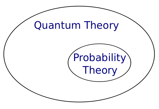
The idea is that quantum theory generalizes classical probability theory by considering observables that don't commute.

That's perfectly valid, but we've been exploring an alternative view in this series. Here quantum theory doesn't subsume probability theory, but they intersect:

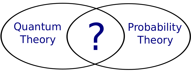
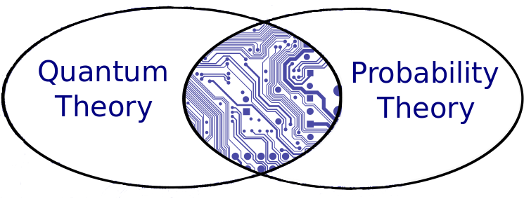
What goes in the middle you might ask? As odd as it might sound at first, John showed in Part 16 that electrical circuits made of resistors constitute the intersection!

For example, a circuit like this:

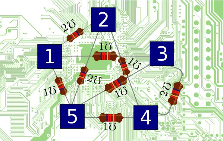
gives rise to a Hamiltonian $H$ that's good both for stochastic mechanics and stochastic mechanics. Indeed, he found that the power dissipated by a circuit made of resistors is related to the familiar quantum theory concept known as the expectation value of the Hamiltonian!

power = - 2 ⟨ ψ, H ψ ⟩

Oh—and you might think we made a mistake and wrote our Ω (ohm) symbols upside down. We didn't. It happens that ℧ is the symbol for a 'mho'—a unit of conductance that's the reciprocal of an ohm. Check out Part 16 for the details.

Stochastic mechanics versus quantum mechanics

Let's recall how states, time evolution, symmetries and observables work in the two theories. Today we'll fix a basis for our vector space of states, and we'll assume it's finite-dimensional so that all vectors have $n$ components over either the complex numbers $C$ or the reals $R$ . In other words, we'll treat our space as either $C^{n}$ or $R^{n}$ . In this fashion, linear operators that map such spaces to themselves will be represented as square matrices.

Vectors will be written as $ψ_{i}$ where the index $i$ runs from 1 to $n$ , and we think of each choice of the index as a state of our system—but since we'll be using that word in other ways too, let's call it a configuration. It's just a basic way our system can be.

States

Besides the configurations $i = 1, \dots, n$ , we have more general states that tell us the probability or amplitude of finding our system in one of these configurations:

• Stochastic states are $n$ -tuples of nonnegative real numbers:

ψ_{i} \in R^{+}

The probability of finding the system in the $i$ th configuration is defined to be $ψ_{i}$ . For these probabilities to sum to one, $ψ_{i}$ needs to be normalized like this:

\sum_{i} ψ_{i} = 1

or in the notation we're using in these articles:

⟨ ψ ⟩ = 1

where we define

⟨ ψ ⟩ = \sum_{i} ψ_{i}

• Quantum states are $n$ -tuples of complex numbers:

ψ_{i} \in C

The probability of finding a state in the $i$ th configuration is defined to be $| ψ (x) |^{2}$ . For these probabilities to sum to one, $ψ$ needs to be normalized like this:

\sum_{i} | ψ_{i} |^{2} = 1

or in other words

⟨ ψ, ψ ⟩ = 1

where the inner product of two vectors $ψ$ and $ϕ$ is defined by

⟨ ψ, ϕ ⟩ = \sum_{i} {\overset{―}{ψ}}_{i} ϕ_{i}

Now, the usual way to turn a quantum state $ψ$ into a stochastic state is to take the absolute value of each number $ψ_{i}$ and then square it. However, if the numbers $ψ_{i}$ happen to be nonnegative, we can also turn $ψ$ into a stochastic state simply by multiplying it by a number to ensure $⟨ ψ ⟩ = 1$ .

This is very unorthodox, but it lets us evolve the same vector $ψ$ either stochastically or quantum-mechanically, using the recipes I'll describe next. In physics jargon these correspond to evolution in 'real time' and 'imaginary time'. But don't ask me which is which: from a quantum viewpoint stochastic mechanics uses imaginary time, but from a stochastic viewpoint it's the other way around!

Time evolution

Time evolution works similarly in stochastic and quantum mechanics, but with a few big differences:

• In stochastic mechanics the state changes in time according to the master equation:

\frac{d}{d t} ψ (t) = H ψ (t)

which has the solution

ψ (t) = \exp (t H) ψ (0)

• In quantum mechanics the state changes in time according to Schrödinger's equation:

\frac{d}{d t} ψ (t) = - i H ψ (t)

which has the solution

ψ (t) = \exp (- i t H) ψ (0)

The operator $H$ is called the Hamiltonian. The properties it must have depend on whether we're doing stochastic mechanics or quantum mechanics:

• We need $H$ to be infinitesimal stochastic for time evolution given by $\exp (t H)$ to send stochastic states to stochastic states. In other words, we need that (i) its columns sum to zero and (ii) its off-diagonal entries are real and nonnegative:

\sum_{i} H_{i j} = 0

i \neq j \Rightarrow H_{i j} \geq 0

• We need $H$ to be self-adjoint for time evolution given by $\exp (- i t H)$ to send quantum states to quantum states. So, we need

H = H^{†}

where we recall that the adjoint of a matrix is the conjugate of its transpose:

(H^{†})_{i j} := {\overset{―}{H}}_{j i}

We are concerned with the case where the operator $H$ generates both a valid quantum evolution and also a valid stochastic one:

• $H$ is a Dirichlet operator if it's both self-adjoint and infinitesimal stochastic. We will soon go further and zoom in on this intersection! But first let's finish our review.

Symmetries

As John explained in Part 12, besides states and observables we need symmetries, which are transformations that map states to states. These include the evolution operators which we only briefly discussed in the preceding subsection.

• A linear map $U$ that sends quantum states to quantum states is called an isometry, and isometries are characterized by this property:

U^{†} U = 1

• A linear map $U$ that sends stochastic states to stochastic states is called a stochastic operator, and stochastic operators are characterized by these properties:

\sum_{i} U_{i j} = 1

and

U_{i j} \geq 0

A notable difference here is that in our finite-dimensional situation, isometries are always invertible, but stochastic operators may not be! If $U$ is an $n \times n$ matrix that's an isometry, $U^{†}$ is its inverse. So, we also have

U U^{†} = 1

and we say $U$ is unitary. But if $U$ is stochastic, it may not have an inverse—and even if it does, its inverse is rarely stochastic. This explains why in stochastic mechanics time evolution is often not reversible, while in quantum mechanics it always is.

Puzzle 1. Suppose $U$ is a stochastic $n \times n$ matrix whose inverse is stochastic. What are the possibilities for $U$ ?

It is quite hard for an operator to be a symmetry in both stochastic and quantum mechanics, especially in our finite-dimensional situation:

Puzzle 2. Suppose $U$ is an $n \times n$ matrix that is both stochastic and unitary. What are the possibilities for $U$ ?

Observables

'Observables' are real-valued quantities that can be measured, or predicted, given a specific theory.

• In quantum mechanics, an observable is given by a self-adjoint matrix $O$ , and the expected value of the observable $O$ in the quantum state $ψ$ is

⟨ ψ, O ψ ⟩ = \sum_{i, j} {\overset{―}{ψ}}_{i} O_{i j} ψ_{j}

• In stochastic mechanics, an observable $O$ has a value $O_{i}$ in each configuration $i$ , and the expected value of the observable $O$ in the stochastic state $ψ$ is

⟨ O ψ ⟩ = \sum_{i} O_{i} ψ_{i}

We can turn an observable in stochastic mechanics into an observable in quantum mechanics by making a diagonal matrix whose diagonal entries are the numbers $O_{i}$ .

From graphs to matrices

Back in Part 16, John explained how a graph with positive numbers on its edges gives rise to a Hamiltonian in both quantum and stochastic mechanics—in other words, a Dirichlet operator.

Here's how this works. We'll consider simple graphs: graphs without arrows on their edges, with at most one edge from one vertex to another, and with no edge from a vertex to itself. And we'll only look at graphs with finitely many vertices and edges. We'll assume each edge is labelled by a positive number, like this:

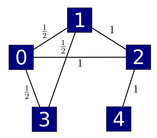
If our graph has $n$ vertices, we can create an $n \times n$ matrix $A$ where $A_{i j}$ is the number labelling the edge from $i$ to $j$ , if there is such an edge, and 0 if there's not. This matrix is symmetric, with real entries, so it's self-adjoint. So $A$ is a valid Hamiltonian in quantum mechanics.

How about stochastic mechanics? Remember that a Hamiltonian in stochastic mechanics needs to be 'infinitesimal stochastic'. So, its off-diagonal entries must be nonnegative, which is indeed true for our $A$ , but also the sums of its columns must be zero, which is not true when our $A$ is nonzero.

But now comes the best news you've heard all day: we can improve $A$ to a stochastic operator in a way that is completely determined by $A$ itself! This is done by subtracting a diagonal matrix $L$ whose entries are the sums of the columns of $A$ :

L_{i i} = \sum_{i} A_{i j}

i \neq j \Rightarrow L_{i j} = 0

It's easy to check that

H = A - L

is still self-adjoint, but now also infinitesimal stochastic. So, it's a Dirichlet operator: a good Hamiltonian for both stochastic and quantum mechanics!

In Part 16, we saw a bit more: every Dirichlet operator arises this way. It's easy to see. You just take your Dirichlet operator and make a graph with one edge for each nonzero off-diagonal entry. Then you label the edge with this entry. So, Dirichlet operators are essentially the same as finite simple graphs with edges labelled by positive numbers.

Now, a simple graph can consist of many separate 'pieces', called components. Then there's no way for a particle hopping along the edges to get from one component to another, either in stochastic or quantum mechanics. So we might as well focus our attention on graphs with just one component. These graphs are called 'connected'. In other words:

Definition. A simple graph is connected if it is nonempty and there is a path of edges connecting any vertex to any other.

Our goal today is to understand more about Dirichlet operators coming from connected graphs. For this we need to learn the Perron–Frobenius theorem. But let's start with something easier.

Perron's theorem

In quantum mechanics it's good to think about observables that have positive expected values:

⟨ ψ, O ψ ⟩ > 0

for every quantum state $ψ \in C^{n}$ . These are called positive definite. But in stochastic mechanics it's good to think about matrices that are positive in a more naive sense:

Definition. An $n \times n$ real matrix $T$ is positive if all its entries are positive:

T_{i j} > 0

for all $1 \leq i, j \leq n$ .

Similarly:

Definition. A vector $ψ \in R^{n}$ is positive if all its components are positive:

ψ_{i} > 0

for all $1 \leq i \leq n$ .

We'll also define nonnegative matrices and vectors in the same way, replacing $> 0$ by $\geq 0$ . A good example of a nonnegative vector is a stochastic state.

In 1907, Perron proved the following fundamental result about positive matrices:

Perron's Theorem. Given a positive square matrix $T$ , there is a positive real number $r$ , called the Perron–Frobenius eigenvalue of $T$ , such that $r$ is an eigenvalue of $T$ and any other eigenvalue $λ$ of $T$ has $| λ | < r$ . Moreover, there is a positive vector $ψ \in R^{n}$ with $T ψ = r ψ$ . Any other vector with this property is a scalar multiple of $ψ$ . Furthermore, any nonnegative vector that is an eigenvector of $T$ must be a scalar multiple of $ψ$ .

In other words, if $T$ is positive, it has a unique eigenvalue with the largest absolute value. This eigenvalue is positive. Up to a constant factor, it has an unique eigenvector. We can choose this eigenvector to be positive. And then, up to a constant factor, it's the only nonnegative eigenvector of $T$ .

From matrices to graphs

The conclusions of Perron's theorem don't hold for matrices that are merely nonnegative. For example, these matrices

(\begin{array}{cc} 1 & 0 \\ 0 & 1 \end{array}), (\begin{array}{cc} 0 & 1 \\ 0 & 0 \end{array})

are nonnegative, but they violate lots of the conclusions of Perron's theorem.

Nonetheless, in 1912 Frobenius published an impressive generalization of Perron's result. In its strongest form, it doesn't apply to all nonnegative matrices; only to those that are 'irreducible'. So, let us define those.

We've seen how to build a matrix from a graph. Now we need to build a graph from a matrix! Suppose we have an $n \times n$ matrix $T$ . Then we can build a graph $G_{T}$ with $n$ vertices where there is an edge from the $i$ th vertex to the $j$ th vertex if and only if $T_{i j} \neq 0$ .

But watch out: this is a different kind of graph! It's a directed graph, meaning the edges have directions, there's at most one edge going from any vertex to any vertex, and we do allow an edge going from a vertex to itself. There's a stronger concept of 'connectivity' for these graphs:

Definition. A directed graph is strongly connected if there is a directed path of edges going from any vertex to any other vertex.

So, you have to be able to walk along edges from any vertex to any other vertex, but always following the direction of the edges! Using this idea we define irreducible matrices:

Definition. A nonnegative square matrix $T$ is irreducible if its graph $G_{T}$ is strongly connected.

The Perron–Frobenius theorem

Now we are ready to state:

The Perron-Frobenius Theorem. Given an irreducible nonnegative square matrix $T$ , there is a positive real number $r$ , called the Perron-.Frobenius eigenvalue of $T$ , such that $r$ is an eigenvalue of $T$ and any other eigenvalue $λ$ of $T$ has $| λ | \leq r$ . Moreover, there is a positive vector $ψ \in R^{n}$ with $T ψ = r ψ$ . Any other vector with this property is a scalar multiple of $ψ$ . Furthermore, any nonnegative vector that is an eigenvector of $T$ must be a scalar multiple of $ψ$ .

The only conclusion of this theorem that's weaker than those of Perron's theorem is that there may be other eigenvalues with $| λ | = r$ . For example, this matrix is irreducible and nonnegative:

(\begin{array}{cc} 0 & 1 \\ 1 & 0 \end{array})

Its Perron–Frobenius eigenvalue is 1, but it also has -1 as an eigenvalue. In general, Perron–Frobenius theory says quite a lot about the other eigenvalues on the circle $| λ | = r,$ but we won't need that fancy stuff here.

Perron–Frobenius theory is useful in many ways, from highbrow math to ranking football teams. We'll need it not just today but also later in this series. There are many books and other sources of information for those that want to take a closer look at this subject. If you're interested, you can search online or take a look at these:

Dimitrious Noutsos, Perron Frobenius theory and some extensions, 2008. (Includes proofs of the basic theorems.)

V. S. Sunder, Perron Frobenius theory, 18 December 2009. (Includes applications to graph theory, Markov chains and von Neumann algebras.)

Stephen Boyd, Lecture 17: Perron Frobenius theory, Winter 2008-2009. (Includes a max-min characterization of the Perron–Frobenius eigenvalue and applications to Markov chains, economics, population growth and power control.)

I have not taken a look myself, but if anyone is interested and can read German, the original work appears here:

Oskar Perron, Zur Theorie der Matrizen, Math. Ann. 64 (1907), 248–263.

Georg Frobenius, Über Matrizen aus nicht negativen Elementen, S.-B. Preuss Acad. Wiss. Berlin (1912), 456–477.

And, of course, there's this:

Wikipedia, Perron–Frobenius theorem.

It's quite good.

Irreducible Dirichlet operators

Now comes the payoff. We saw how to get a Dirichlet operator $H$ from any finite simple graph with edges labelled by positive numbers. Now let's apply Perron–Frobenius theory to prove our thesis.

Unfortunately, the matrix $H$ is rarely nonnegative. If you remember how we built it, you'll see its off-diagonal entries will always be nonnegative... but its diagonal entries can be negative.

Luckily, we can fix this just by adding a big enough multiple of the identity matrix to $H$ ! The result is a nonnegative matrix

T = H + c I

where $c > 0$ is some large number. This matrix $T$ has the same eigenvectors as $H$ . The off-diagonal matrix entries of $T$ are the same as those of $H$ , so $T_{i j}$ is nonzero for $i \neq j$ exactly when the graph we started with has an edge from $i$ to $j$ . So, for $i \neq j$ , the graph $G_{T}$ will have an directed edge going from $i$ to $j$ precisely when our original graph had an edge from $i$ to $j$ . And that means that if our original graph was connected, $G_{T}$ will be strongly connected. Thus, by definition, the matrix $T$ is irreducible!

Since $T$ is nonnegative and irreducible, the Perron–Frobenius theorem swings into action and we conclude:

Lemma. Suppose $H$ is the Dirichlet operator coming from a connected finite simple graph with edges labelled by positive numbers. Then the eigenvalues of $H$ are real. Let $λ$ be the largest eigenvalue. Then there is a positive vector $ψ \in R^{n}$ with $H ψ = λ ψ$ . Any other vector with this property is a scalar multiple of $ψ$ . Furthermore, any nonnegative vector that is an eigenvector of $H$ must be a scalar multiple of $ψ$ .

Proof. The eigenvalues of $H$ are real since $H$ is self-adjoint. Notice that if $r$ is the Perron–Frobenius eigenvalue of $T = H + c I$ and

T ψ = r ψ

then

H ψ = (r - c) ψ

By the Perron–Frobenius theorem the number $r$ is positive, and it has the largest absolute value of any eigenvalue of $T$ . Thanks to the subtraction, the eigenvalue $r - c$ may not have the largest absolute value of any eigenvalue of $H$ . It is, however, the largest eigenvalue of $H$ , so we take this as our $λ$ . The rest follows from the Perron–Frobenius theorem. █

But in fact we can improve this result, since the largest eigenvalue $λ$ is just zero. Let's also make up a definition, to make our result sound more slick:

Definition. A Dirichlet operator is irreducible if it comes from a connected finite simple graph with edges labelled by positive numbers.

This meshes nicely with our earlier definition of irreducibility for nonnegative matrices. Now:

Theorem. Suppose $H$ is an irreducible Dirichlet operator. Then $H$ has zero as its largest real eigenvalue. There is a positive vector $ψ \in R^{n}$ with $H ψ = 0$ . Any other vector with this property is a scalar multiple of $ψ$ . Furthermore, any nonnegative vector that is an eigenvector of $H$ must be a scalar multiple of $ψ$ .

Proof. Choose $λ$ as in the Lemma, so that $H ψ = λ ψ$ . Since $ψ$ is positive we can normalize it to be a stochastic state:

\sum_{i} ψ_{i} = 1

Since $H$ is a Dirichlet operator, $\exp (t H)$ sends stochastic states to stochastic states, so

\sum_{i} (\exp (t H) ψ)_{i} = 1

for all $t \geq 0$ . On the other hand,

\sum_{i} (\exp (t H) ψ)_{i} = \sum_{i} e^{t λ} ψ_{i} = e^{t λ}

so we must have $λ = 0$ . █

What's the point of all this? One point is that there's a unique stochastic state $ψ$ that's an equilibrium state: since $H ψ = 0$ , it doesn't change with time. It's also globally stable: since all the other eigenvalues of $H$ are negative, all other stochastic states converge to this one as time goes forward.

An example

There are many examples of irreducible Dirichlet operators. For instance, in Part 15 we talked about graph Laplacians. The Laplacian of a connected simple graph is always irreducible. But let us try a different sort of example, coming from the picture of the resistors we saw earlier:

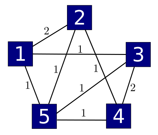
Let's create a matrix $A$ whose entry $A_{i j}$ is the number labelling the edge from $i$ to $j$ if there is such an edge, and zero otherwise:

A = (\begin{array}{ccccc} 0 & 2 & 1 & 0 & 1 \\ 2 & 0 & 0 & 1 & 1 \\ 1 & 0 & 0 & 2 & 1 \\ 0 & 1 & 2 & 0 & 1 \\ 1 & 1 & 1 & 1 & 0 \end{array})

Remember how the game works. The matrix $A$ is already a valid Hamiltonian for quantum mechanics, since it's self adjoint. However, to get a valid Hamiltonian for both stochastic and quantum mechanics—in other words, a Dirichlet operator—we subtract the diagonal matrix $L$ whose entries are the sums of the columns of $A .$ In this example it just so happens that the column sums are all 4, so $L = 4 I,$ and our Dirichlet operator is

H = A - 4 I = (\begin{array}{ccccc} - 4 & 2 & 1 & 0 & 1 \\ 2 & - 4 & 0 & 1 & 1 \\ 1 & 0 & - 4 & 2 & 1 \\ 0 & 1 & 2 & - 4 & 1 \\ 1 & 1 & 1 & 1 & - 4 \end{array})

We've set up this example so it's easy to see that the vector $ψ = (1, 1, 1, 1, 1)$ has

H ψ = 0

So, this is the unique eigenvector for the eigenvalue 0. We can use Mathematica to calculate the remaining eigenvalues of $H$ . The set of eigenvalues is

{0, - 7, - 8, - 8, - 3}

As we expect from our theorem, the largest real eigenvalue is 0. By design, the eigenstate associated to this eigenvalue is

| v_{0} ⟩ = (1, 1, 1, 1, 1)

(This funny notation for vectors is common in quantum mechanics, so don't worry about it.) All the other eigenvectors fail to be nonnegative, as predicted by the theorem. They are:

| v_{1} ⟩ = (1, - 1, - 1, 1, 0),

| v_{2} ⟩ = (- 1, 0, - 1, 0, 2),

| v_{3} ⟩ = (- 1, 1, - 1, 1, 0),

| v_{4} ⟩ = (- 1, - 1, 1, 1, 0) .

To compare the quantum and stochastic states, consider first $| v_{0} ⟩$ . This is the only eigenvector that can be normalized to a stochastic state. Remember, a stochastic state must have nonnegative components. This rules out $| v_{1} ⟩$ through to $| v_{4} ⟩$ as valid stochastic states, no matter how we normalize them! However, these are allowed as states in quantum mechanics, once we normalize them correctly. For a stochastic system to be in a state other than the Perron–Frobenius state, it must be a linear combination of least two eigenstates. For instance,

ψ_{a} = (1 - a) | v_{0} ⟩ + a | v_{1} ⟩

can be normalized to give stochastic state only if $0 \leq a \leq \frac{1}{2}$ .

And, it's easy to see that it works this way for any irreducible Dirichlet operator, thanks to our theorem. So, our thesis has been proved true!

Puzzles on irreducibility

Let us conclude with a couple more puzzles. There are lots of ways to characterize irreducible nonnegative matrices; we don't need to mention graphs. Here's one:

Puzzle 3. Let $T$ be a nonnegative $n \times n$ matrix. Show that $T$ is irreducible if and only if for all $i, j \geq 0$ , $(T^{m})_{i j} > 0$ for some natural number $m$ .

You may be confused because today we explained the usual concept of irreducibility for nonnegative matrices, but also defined a concept of irreducibility for Dirichlet operators. Luckily there's no conflict: Dirichlet operators aren't nonnegative matrices, but if we add a big multiple of the identity to a Dirichlet operator it becomes a nonnegative matrix, and then:

Puzzle 4. Show that a Dirichlet operator $H$ is irreducible if and only if the nonnegative operator $H + c I$ (where $c$ is any sufficiently large constant) is irreducible.

Irreducibility is also related to the nonexistence of interesting conserved quantities. In Part 11 we saw a version of Noether's Theorem for stochastic mechanics. Remember that an observable $O$ in stochastic mechanics assigns a number $O_{i}$ to each configuration $i = 1, \dots, n$ . We can make a diagonal matrix with $O_{i}$ as its diagonal entries, and by abuse of language we call this $O$ as well. Then we say $O$ is a conserved quantity for the Hamiltonian $H$ if the commutator $[O, H] = O H - H O$ vanishes.

Puzzle 5. Let $H$ be a Dirichlet operator. Show that $H$ is irreducible if and only if every conserved quantity $O$ for $H$ is a constant, meaning that for some $c \in R$ we have $O_{i} = c$ for all $i$ . (Hint: examine the proof of Noether's theorem.)

In fact this works more generally:

Puzzle 6. Let $H$ be an infinitesimal stochastic matrix. Show that $H + c I$ is an irreducible nonnegative matrix for all sufficiently large $c$ if and only if every conserved quantity $O$ for $H$ is a constant.

You can also read comments on Azimuth, and make your own comments or ask questions there!