

|
|
|
|
We've been looking at reaction networks, and we're getting ready to find equilibrium solutions of the equations they give. To do this, we'll need to connect them to another kind of network we've studied. A reaction network is something like this:
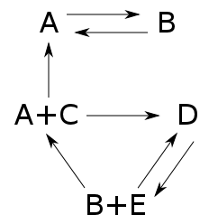
It's a bunch of complexes, which are sums of basic building-blocks called species, together with arrows called transitions going between the complexes. If we know a number for each transition describing the rate at which it occurs, we get an equation called the 'rate equation'. This describes how the amount of each species changes with time. We've been talking about this equation ever since the start of this series! Last time, we wrote it down in a new very compact form:
$$ \displaystyle{ \frac{d x}{d t} = Y H x^Y } $$
Here $ x$ is a vector whose components are the amounts of each species, while $ H$ and $ Y$ are certain matrices.
But now suppose we forget how each complex is made of species! Suppose we just think of them as abstract things in their own right, like numbered boxes:
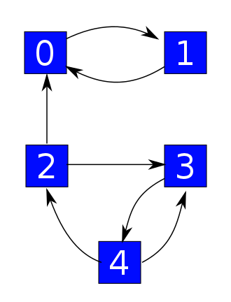
We can use these boxes to describe states of some system. The arrows still describe transitions, but now we think of these as ways for the system to hop from one state to another. Say we know a number for each transition describing the probability per time at which it occurs:
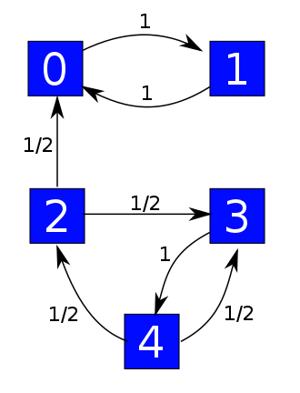
Then we get a 'Markov process' — or in other words, a random walk where our system hops from one state to another. If $\psi$ is the probability distribution saying how likely the system is to be in each state, this Markov process is described by this equation:
$$ \displaystyle{ \frac{d \psi}{d t} = H \psi } $$
This is simpler than the rate equation, because it's linear. But the matrix $H$ is the same—we'll see that explicitly later on today.
What's the point? Well, our ultimate goal is to prove the deficiency zero theorem, which gives equilibrium solutions of the rate equation. That means finding $x$ with
$$ Y H x^Y = 0 $$
Today we'll find all equilibria for the Markov process, meaning all $\psi$ with
$$ H \psi = 0 $$
Then next time we'll show some of these have the form
$$ \psi = x^Y $$
So, we'll get
$$ H x^Y = 0 $$
and thus
$$ Y H x^Y = 0 $$
as desired!
So, let's get to to work.
We've been looking at stochastic reaction networks, which are things like this:
However, we can build a Markov process starting from just part of this information:
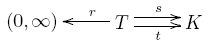
Let's call this thing a 'graph with rates', for lack of a better name. We've been calling the things in $K$ 'complexes', but now we'll think of them as 'states'. So:
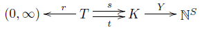
Definition. A graph with rates consists of:
• a finite set of states $K$,
• a finite set of transitions $T$,
• a map $r: T \to (0,\infty)$ giving a rate constant for each transition,
• source and target maps $s,t : T \to K$ saying where each transition starts and ends.
Starting from this, we can get a Markov process describing how a probability distribution $\psi$ on our set of states will change with time. As usual, this Markov process is described by a master equation:
$$ \displaystyle{ \frac{d \psi}{d t} = H \psi } $$
for some Hamiltonian:
$$ H : \mathbb{R}^K \to \mathbb{R}^K $$
What is this Hamiltonian, exactly? Let's think of it as a matrix where $H_{i j}$ is the probability per time for our system to hop from the state $j$ to the state $i$. This looks backwards, but don't blame me—blame the guys who invented the usual conventions for matrix algebra. Clearly if $i \ne j$ this probability per time should be the sum of the rate constants of all transitions going from $j$ to $i$:
$$ i \ne j \quad \Rightarrow \quad H_{i j} = \sum_{\tau: j \to i} r(\tau) $$
where we write $\tau: j \to i$ when $\tau$ is a transition with source $j$ and target $i$.
Now, we saw in Part 11 that for a probability distribution to remain a probability distribution as it evolves in time according to the master equation, we need $H$ to be infinitesimal stochastic: its off-diagonal entries must be nonnegative, and the sum of the entries in each column must be zero.
The first condition holds already, and the second one tells us what the diagonal entries must be. So, we're basically done describing $H$. But we can summarize it this way:
Puzzle 1. Think of $\mathbb{R}^K$ as the vector space consisting of finite linear combinations of elements $\kappa \in K$. Then show
$$ H \kappa = \sum_{s(\tau) = \kappa} r(\tau) (t(\tau) - s(\tau)) $$
Now we'll classify equilibrium solutions of the master equation, meaning $\psi \in \mathbb{R}^K$ with
$$ H \psi = 0 $$
We'll do only do this when our graph with rates is 'weakly reversible'. This concept doesn't actually depend on the rates, so let's be general and say:
Definition. A graph is weakly reversible if for every edge $\tau : i \to j$, there is directed path going back from $j$ to $i$, meaning that we have edges
$$ \tau_1 : j \to j_1 , \quad \tau_2 : j_1 \to j_2 , \quad \dots, \quad \tau_n: j_{n-1} \to i $$
This graph with rates is not weakly reversible:
but this one is:
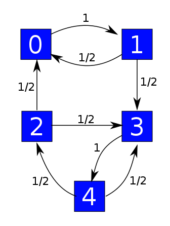
The good thing about the weakly reversible case is that we get one equilibrium solution of the master equation for each component of our graph, and all equilibrium solutions are linear combinations of these. This is not true in general! For example, this guy is not weakly reversible:
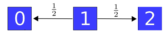
It has only one component, but the master equation has two linearly independent equilibrium solutions: one that vanishes except at the state 0, and one that vanishes except at the state 2.
The idea of a 'component' is supposed to be fairly intuitive — our graph falls apart into pieces called components — but we should make it precise. As explained in Part 21, the graphs we're using here are directed multigraphs, meaning things like
$$ s, t : E \to V $$
where $E$ is the set of edges (our transitions) and $V$ is the set of vertices (our states). There are actually two famous concepts of 'component' for graphs of this sort: 'strongly connected' components and 'connected' components. We only need connected components, but let me explain both concepts, in a feeble attempt to slake your insatiable thirst for knowledge.
Two vertices $i$ and $j$ of a graph lie in the same strongly connected component iff you can find a directed path of edges from $i$ to $j$ and also one from $j$ back to $i$.
Remember, a directed path from $i$ to $j$ looks like this:
$$ i \to a \to b \to c \to j $$
Here's a path from $x$ to $y$ that is not directed:
$$ i \to a \leftarrow b \to c \to j $$
and I hope you can write down the obvious but tedious definition of an 'undirected path', meaning a path made of edges that don't necessarily point in the correct direction. Given that, we say two vertices $i$ and $j$ lie in the same connected component iff you can find an undirected path going from $i$ to $j$. In this case, there will automatically also be an undirected path going from $j$ to $i$.
For example, $i$ and $j$ lie in the same connected component here, but not the same strongly connected component:
$$ i \to a \leftarrow b \to c \to j $$
Here's a graph with one connected component and 3 strongly connected components, which are marked in blue:
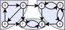
For the theory we're looking at now, we only care about connected components, not strongly connected components! However:
Puzzle 2. Show that for weakly reversible graph, the connected components are the same as the strongly connected components.
With these definitions out of way, we can state today's big theorem:
Theorem. Suppose $H$ is the Hamiltonian of a weakly reversible graph with rates:
Then for each connected component $C \subseteq K$, there exists a unique probability distribution $\psi_C \in \mathbb{R}^K$ that is positive on that component, zero elsewhere, and is an equilibrium solution of the master equation:
$$ H \psi_C = 0 $$
Moreover, these probability distributions $\psi_C$ form a basis for the space of equilibrium solutions of the master equation. So, the dimension of this space is the number of components of $K$.
Proof. We start by assuming our graph has one connected component. We use the Perron–Frobenius theorem, as explained in Part 20. This applies to 'nonnegative' matrices, meaning those whose entries are all nonnegative. That is not true of $H$ itself, but only its diagonal entries can be negative, so if we choose a large enough number $c > 0$, $H + c I$ will be nonnegative.
Since our graph is weakly reversible and has one connected component, it follows straight from the definitions that the operator $H + c I$ will also be 'irreducible' in the sense of Part 20. The Perron–Frobenius theorem then swings into action, and we instantly conclude several things.
First, $H + c I$ has a positive real eigenvalue $r$ such that any other eigenvalue, possibly complex, has absolute value $\le r$. Second, there is an eigenvector $\psi$ with eigenvalue $r$ and all positive components. Third, any other eigenvector with eigenvalue $r$ is a scalar multiple of $\psi$.
Subtracting $c$, it follows that $\lambda = r - c$ is the eigenvalue of $H$ with the largest real part. We have $H \psi = \lambda \psi$, and any other vector with this property is a scalar multiple of $\psi$.
We can show that in fact $\lambda = 0$. To do this we copy an argument from Part 20. First, since $\psi$ is positive we can normalize it to be a probability distribution:
$$ \displaystyle{ \sum_{i \in K} \psi_i = 1 } $$
Since $H$ is infinitesimal stochastic, $\exp(t H)$ sends probability distributions to probability distributions:
$$ \displaystyle{ \sum_{i \in K} (\exp(t H) \psi)_i = 1 } $$
for all $t \ge 0$. On the other hand,
$$ \sum_{i \in K} (\exp(t H)\psi)_i = \sum_{i \in K} e^{t \lambda} \psi_i = e^{t \lambda} $$
so we must have $\lambda = 0$.
We conclude that when our graph has one connected component, there is a probability distribution $\psi \in \mathbb{R}^K$ that is positive everywhere and has $H \psi = 0$. Moreover, any $\phi \in \mathbb{R}^K$ with $H \phi = 0$ is a scalar multiple of $\psi$.
When $K$ has several components, the matrix $H$ is block diagonal, with one block for each component. So, we can run the above argument on each component $C \subseteq K$ and get a probability distribution $\psi_C \in \mathbb{R}^K$ that is positive on $C$. We can then check that $H \psi_C = 0$ and that every $\phi \in \mathbb{R}^K$ with $H \phi = 0$ can be expressed as a linear combination of these probability distributions $\psi_C$ in a unique way. █
This result must be absurdly familiar to people who study Markov processes, but I haven't bothered to look up a reference yet. Do you happen to know a good one? I'd like to see one that generalizes this theorem to graphs that aren't weakly reversible. I think I see how it goes. We don't need that generalization right now, but it would be good to have around.
One last small piece of business: last time I showed you a very slick formula for the Hamiltonian $H$. I'd like to prove it agrees with the formula I gave this time.
We start with any graph with rates:
We extend $s$ and $t$ to linear maps between vector spaces:
We define the boundary operator just as we did last time:
$$ \partial = t - s $$
Then we put an inner product on the vector spaces $\mathbb{R}^T$ and $\mathbb{R}^K$. So, for $\mathbb{R}^K$ we let the elements of $K$ be an orthonormal basis, but for $\mathbb{R}^T$ we define the inner product in a more clever way involving the rate constants:
$$ \displaystyle{ \langle \tau, \tau' \rangle = \frac{1}{r(\tau)} \delta_{\tau, \tau'} } $$
where $\tau, \tau' \in T$. These inner products let us define adjoints of the maps $s, t$ and $\partial$, via formulas like this:
$$ \langle s^\dagger \phi, \psi \rangle = \langle \phi, s \psi \rangle $$
Then:
Theorem. The Hamiltonian for a graph with rates is given by
$$ H = \partial s^\dagger $$
Proof. It suffices to check that this formula agrees with the formula for $H$ given in Puzzle 1:
$$ H \kappa = \sum_{s(\tau) = \kappa} r(\tau) (t(\tau) - s(\tau)) $$
Recall that here we are writing $\kappa \in K$ is any the standard basis vectors of $\mathbb{R}^K$. Similarly shall we write things like $\tau$ or $\tau'$ for basis vectors of $\mathbb{R}^T$.
First, we claim that
$$ s^\dagger \kappa = \sum_{\tau: \; s(\tau) = \kappa} r(\tau) \, \tau $$
To prove this it's enough to check that taking the inner products of either sides with any basis vector $\tau'$, we get results that agree. On the one hand:
$$ \begin{array}{ccl} \langle \tau' , s^\dagger \kappa \rangle &=& \langle s \tau', \kappa \rangle \\ \\ &=& \delta_{s(\tau'), \kappa} \end{array} $$
On the other hand, using our clever inner product on $\mathbb{R}^T$ we see that:
$$ \begin{array}{ccl} \displaystyle{ \langle \tau', \sum_{\tau: \; s(\tau) = \kappa} r(\tau) \, \tau \rangle } &=& \sum_{\tau: \; s(\tau) = \kappa} r(\tau) \, \langle \tau', \tau \rangle \\ &=& \sum_{\tau: \; s(\tau) = \kappa} \delta_{\tau', \tau} \\ &=& \delta_{s(\tau'), \kappa} \end{array} $$
where the factor of $1/r(\tau)$ in the inner product on $\mathbb{R}^T$ cancels the visible factor of $r(\tau)$. So indeed the results match.
Using this formula for $s^\dagger \kappa $ we now see that
$$ \begin{array}{ccl} H \kappa &=& \partial s^\dagger \kappa \\ &=& \partial \displaystyle{ \sum_{\tau: \; s(\tau) = \kappa} r(\tau) \, \tau } \\ &=& \displaystyle{ \sum_{\tau: \; s(\tau) = \kappa} r(\tau) \, (t(\tau) - s(\tau)) } \end{array} $$
which is precisely what we want. █
I hope you see through the formulas to their intuitive meaning. As usual, the formulas are just a way of precisely saying something that makes plenty of sense. If $\kappa$ is some state of our Markov process, $ s^\dagger \kappa$ is the sum of all transitions starting at this state, weighted by their rates. Applying $ \partial$ to a transition tells us what change in state it causes. So $ \partial s^\dagger \kappa$ tells us the rate at which things change when we start in the state $ \kappa$. That's why $\partial s^\dagger$ is the Hamiltonian for our Markov process. After all, the Hamiltonian tells us how things change:
$$ \displaystyle{ \frac{d \psi}{d t} = H \psi } $$
Okay, we've got all the machinery in place. Next time we'll prove the deficiency zero theorem!
You can also read comments on Azimuth, and make your own comments or ask questions there!
|
|
|
|